pyfar.dsp¶

Classes:

InterpolateSpectrum(data, method, kind[, ...])

Interpolate an incomplete spectrum to a complete single sided spectrum.

Functions:

`convolve`(signal1, signal2[, mode, method])	Convolve two signals.
`deconvolve`(system_output, system_input[, ...])	Calculate transfer functions by spectral deconvolution of two signals.
`group_delay`(signal[, frequencies, method])	Returns the group delay of a signal in samples.
`kaiser_window_beta`(A)	Return a shape parameter beta to create kaiser window based on desired side lobe suppression in dB.
`linear_phase`(signal, group_delay[, unit])	Set the phase to a linear phase with a specified group delay.
`minimum_phase`(signal[, method, n_fft, pad, ...])	Calculate the minimum phase equivalent of a signal or filter
`pad_zeros`(signal, pad_width[, mode])	Pad a signal with zeros in the time domain.
`phase`(signal[, deg, unwrap])	Returns the phase for a given signal object.
`regularized_spectrum_inversion`(signal, ...)	Invert the spectrum of a signal applying frequency dependent regularization.
`spectrogram`(signal[, window, window_length, ...])	Compute the magnitude spectrum versus time.
`time_shift`(signal, shift[, unit])	Apply a time-shift to a signal.
`time_window`(signal, interval[, window, ...])	Apply time window to signal.
`wrap_to_2pi`(x)	Wraps phase to 2 pi.
`zero_phase`(signal)	Calculate zero phase signal.

class pyfar.dsp.InterpolateSpectrum(data, method, kind, fscale='linear', clip=False, group_delay=None, unit='samples')[source]¶

Bases: object

Interpolate an incomplete spectrum to a complete single sided spectrum.

This is intended to interpolate transfer functions, for example sparse spectra that are defined only at octave frequencies or incomplete spectra from numerical simulations.

Parameters

data (FrequencyData) – Input data to be interpolated. data.fft_norm must be ‘none’.
method (string) –
Specifies the input data for the interpolation

'complex'
Separate interpolation of the real and imaginary part

'magnitude_phase'
Separate interpolation if the magnitude and unwrapped phase values

'magnitude'
Interpolate the magnitude values only. Results in a zero phase signal, which is symmetric around the first sample. This phase response might not be ideal for many applications. Minimum and linear phase responses can be generated with minimum_phase and linear_phase.
kind (tuple) –
Three element tuple ('first', 'second', 'third') that specifies the kind of inter/extrapolation below the lowest frequency (first), between the lowest and highest frequency (second), and above the highest frequency (third).

The individual strings have to be

'zero', slinear, 'quadratic', 'cubic'
Spline interpolation of zeroth, first, second or third order

'previous', 'next'
Simply return the previous or next value of the point

'nearest-up', 'nearest'
Differ when interpolating half-integers (e.g. 0.5, 1.5) in that 'nearest-up' rounds up and 'nearest' rounds down.

The interpolation is done using scipy.interpolate.interp1d.
fscale (string, optional) –

'linear'
Interpolate on a linear frequency axis.

'log'
Interpolate on a logarithmic frequency axis. Note that 0 Hz can not be interpolated on a logarithmic scale because the logarithm of 0 does not exist. Frequencies of 0 Hz are thus replaced by the next highest frequency before interpolation.

The default is 'linear'.
clip (bool, tuple) – The interpolated magnitude response is clipped to the range specified by this two element tuple. E.g., clip=(0, 1) will assure that no values smaller than 0 and larger than 1 occur in the interpolated magnitude response. The clipping is applied after the interpolation. The default is False which does not clip the data.

Returns

interpolator – The interpolator can be called to interpolate the data (see examples below). It returns a Signal and has the following parameters

n_samplesint: Length of the interpolated time signal in samples
sampling_rate: int: Sampling rate of the output signal in Hz
showbool, optional: Show a plot of the input and output data. The default is False.

Return type

InterpolateSpectrum

Examples

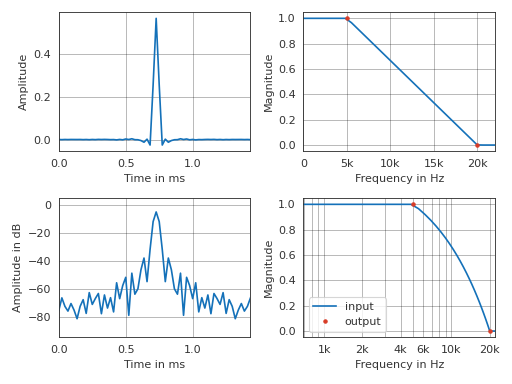
Interpolate a magnitude spectrum, add an artificial linear phase and inspect the results. Note that a similar plot can be created by the interpolator object by signal = interpolator(64, 44100, show=True)

>>> import pyfar as pf
>>> import matplotlib.pyplot as plt
>>> import numpy as np
>>> # generate data
>>> data = pf.FrequencyData([1, 0], [5e3, 20e3])
>>> interpolator = pf.dsp.InterpolateSpectrum(
...     data, 'magnitude', ('nearest', 'linear', 'nearest'))
>>> # interpolate 64 samples at a sampling rate of 44100
>>> signal = interpolator(64, 44100)
>>> # add linear phase
>>> signal = pf.dsp.linear_phase(signal, 32)
>>> # plot input and output data
>>> with pf.plot.context():
>>>     _, ax = plt.subplots(2, 2)
>>>     # time signal (linear and logarithmic amplitude)
>>>     pf.plot.time(signal, ax=ax[0, 0])
>>>     pf.plot.time(signal, ax=ax[1, 0], dB=True)
>>>     # frequency plot (linear x-axis)
>>>     pf.plot.freq(signal, dB=False, freq_scale="linear",
...                  ax=ax[0, 1])
>>>     pf.plot.freq(data, dB=False, freq_scale="linear",
...                  ax=ax[0, 1], c='r', ls='', marker='.')
>>>     ax[0, 1].set_xlim(0, signal.sampling_rate/2)
>>>     # frequency plot (log x-axis)
>>>     pf.plot.freq(signal, dB=False, ax=ax[1, 1], label='input')
>>>     pf.plot.freq(data, dB=False, ax=ax[1, 1],
...                  c='r', ls='', marker='.', label='output')
>>>     min_freq = np.min([signal.sampling_rate / signal.n_samples,
...                        data.frequencies[0]])
>>>     ax[1, 1].set_xlim(min_freq, signal.sampling_rate/2)
>>>     ax[1, 1].legend(loc='best')

(Source code, png, hires.png, pdf)

pyfar.dsp.convolve(signal1, signal2, mode='full', method='overlap_add')[source]¶

Convolve two signals.

Parameters

signal1 (Signal) – The first signal
signal2 (Signal) – The second signal
mode (string, optional) –
A string indicating the size of the output:

'full'
Compute the full discrete linear convolution of the input signals. The output has the length 'signal1.n_samples + signal2.n_samples - 1' (Default).

'cut'
Compute the complete convolution with full and truncate the result to the length of the longer signal.

'cyclic'
The output is the cyclic convolution of the signals, where the shorter signal is zero-padded to fit the length of the longer one. This is done by computing the complete convolution with 'full', adding the tail (i.e., the part that is truncated for mode='cut' to the beginning of the result) and truncating the result to the length of the longer signal.
method (str {'overlap_add', 'fft'}, optional) –
A string indicating which method to use to calculate the convolution:

'overlap_add'
Convolve using the overlap-add algorithm based on scipy.signal.oaconvolve. (Default)

'fft'
Convolve using FFT based on scipy.signal.fftconvolve.

See Notes for more details.

Returns

The convolution result as a Signal object.

Return type

Signal

Notes

The overlap-add method is generally much faster than fft convolution when one signal is much larger than the other, but can be slower when only a few output values are needed or when the signals have a very similar length. For method='overlap_add', integer data will be cast to float.

Examples

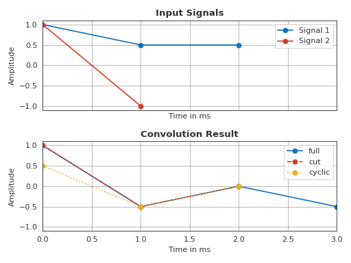
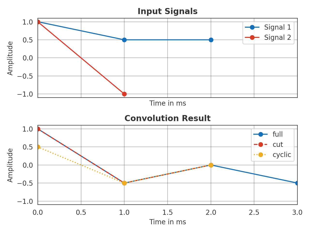
Illustrate the different modes.

>>> import pyfar as pf
>>> s1 = pf.Signal([1, 0.5, 0.5], 1000)
>>> s2 = pf.Signal([1,-1], 1000)
>>> full = pf.dsp.convolve(s1, s2, mode='full')
>>> cut = pf.dsp.convolve(s1, s2, mode='cut')
>>> cyc = pf.dsp.convolve(s1, s2, mode='cyclic')
>>> # Plot input and output
>>> with pf.plot.context():
>>>     fig, ax = plt.subplots(2, 1, sharex=True)
>>>     pf.plot.time(s1, ax=ax[0], label='Signal 1', marker='o')
>>>     pf.plot.time(s2, ax=ax[0], label='Signal 2', marker='o')
>>>     ax[0].set_title('Input Signals')
>>>     ax[0].legend()
>>>     pf.plot.time(full, ax=ax[1], label='full', marker='o')
>>>     pf.plot.time(cut, ax=ax[1], label='cut', ls='--',  marker='o')
>>>     pf.plot.time(cyc, ax=ax[1], label='cyclic', ls=':', marker='o')
>>>     ax[1].set_title('Convolution Result')
>>>     ax[1].set_ylim(-1.1, 1.1)
>>>     ax[1].legend()
>>>     fig.tight_layout()

(Source code, png, hires.png, pdf)

pyfar.dsp.deconvolve(system_output, system_input, fft_length=None, **kwargs)[source]¶

Calculate transfer functions by spectral deconvolution of two signals.

The transfer function $H(\omega)$ is calculated by spectral deconvolution (spectral division).

$H(\omega) = \frac{Y(\omega)}{X(\omega)},$

where $X(\omega)$ is the system input signal and $Y(\omega)$ the system output. Regularized inversion is used to avoid numerical issues in calculating $X(\omega)^{-1} = 1/X(\omega)$ for small values of $X(\omega)$ (see regularized_spectrum_inversion). The system response (transfer function) is thus calculated as

$H(\omega) = Y(\omega)X(\omega)^{-1}.$

For more information, refer to 1.

Parameters

system_output (Signal) – The system output signal (e.g., recorded after passing a device under test). The system output signal is zero padded, if it is shorter than the system input signal.
system_input (Signal) – The system input signal (e.g., used to perform a measurement). The system input signal is zero padded, if it is shorter than the system output signal.
fft_length (int or None) – The length the signals system_output and system_input are zero padded to before deconvolving. The default is None. In this case only the shorter signal is padded to the length of the longer signal, no padding is applied when both signals have the same length.
kwargs (key value arguments) – Key value arguments to control the inversion of $H(\omega)$ are passed to to regularized_spectrum_inversion.

Returns

system_response – The resulting signal after deconvolution, representing the system response (the transfer function). The fft_norm of is set to 'none'.

Return type

Signal

References

1: S. Mueller and P. Masserani “Transfer function measurement with sweeps. Directors cut.” J. Audio Eng. Soc. 49(6):443-471, (2001, June).

pyfar.dsp.group_delay(signal, frequencies=None, method='fft')[source]¶

Returns the group delay of a signal in samples.

Parameters

signal (Signal) – An audio signal object from the pyfar signal class
frequencies (array-like) – Frequency or frequencies in Hz at which the group delay is calculated. The default is None, in which case signal.frequencies is used.
method ('scipy', 'fft', optional) – Method to calculate the group delay of a Signal. Both methods calculate the group delay using the method presented in 2 avoiding issues due to discontinuities in the unwrapped phase. Note that the scipy version additionally allows to specify frequencies for which the group delay is evaluated. The default is 'fft', which is faster.

Returns

group_delay – Frequency dependent group delay in samples. The array is flattened if a single channel signal was passed to the function.

Return type

numpy array

References

2: https://www.dsprelated.com/showarticle/69.php

pyfar.dsp.kaiser_window_beta(A)[source]¶

Return a shape parameter beta to create kaiser window based on desired side lobe suppression in dB.

This function can be used to call time_window with window=('kaiser', beta).

Parameters: A (float) – Side lobe suppression in dB
Returns: beta – Shape parameter beta after 3, Eq. 7.75
Return type: float

References

3: A. V. Oppenheim and R. W. Schafer, Discrete-time signal processing, Third edition, Upper Saddle, Pearson, 2010.

pyfar.dsp.linear_phase(signal, group_delay, unit='samples')[source]¶

Set the phase to a linear phase with a specified group delay.

The linear phase signal is computed as

$H_{\mathrm{lin}} = |H| \mathrm{e}^{-j \omega \tau}\,,$

with $H$ the complex spectrum of the input data, $|\cdot|$ the absolute values, $\omega$ the frequency in radians and $\tau$ the group delay in seconds.

Parameters

signal (Signal) – input data
group_delay (float, array like) – The desired group delay of the linear phase signal according to unit. A reasonable value for most cases is signal.n_samples / 2 samples, which results in a time signal that is symmetric around the center. If group delay is a list or array it must broadcast with the channel layout of the signal (signal.cshape).
unit (string, optional) – Unit of the group delay. Can be 'samples' or 's' for seconds. The default is 'samples'.

Returns

signal – linear phase copy of the input data

Return type

Signal

pyfar.dsp.minimum_phase(signal, method='homomorphic', n_fft=None, pad=False, return_magnitude_ratio=False)[source]¶

Calculate the minimum phase equivalent of a signal or filter

Parameters

signal (Signal) – The linear phase filter.
method (str, optional) –
The method:

’homomorphic’ (default)
This method works best with filters with an odd number of taps, and the resulting minimum phase filter will have a magnitude response that approximates the square root of the the original filter’s magnitude response.

’hilbert’
This method is designed to be used with equi-ripple filters with unity or zero gain regions.
n_fft (int, optional) –
The FFT length used for calculating the cepstrum. Should be at least a few times larger than the signal length. The default is None, resulting in an FFT length of:

n_fft = 2 ** int(np.ceil(np.log2(2*(signal.n_samples - 1) / 0.01)))
pad (bool, optional) – If pad is True, the resulting signal will be padded to the same length as the input. If pad is False the resulting minimum phase representation is of length signal.n_samples/2+1. The default is False
return_magnitude_ratio (bool, optional) – If True, the ratio between the linear phase (input) and the minimum phase (output) filters is returned. See the examples for further information. The default is False.

Returns

signal_minphase (Signal) – The minimum phase version of the filter.
magnitude_ratio (FrequencyData) – The ratio between the (normalized) magnitude spectra of the linear phase and the minimum phase versions of the filter.

Examples

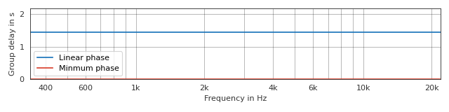
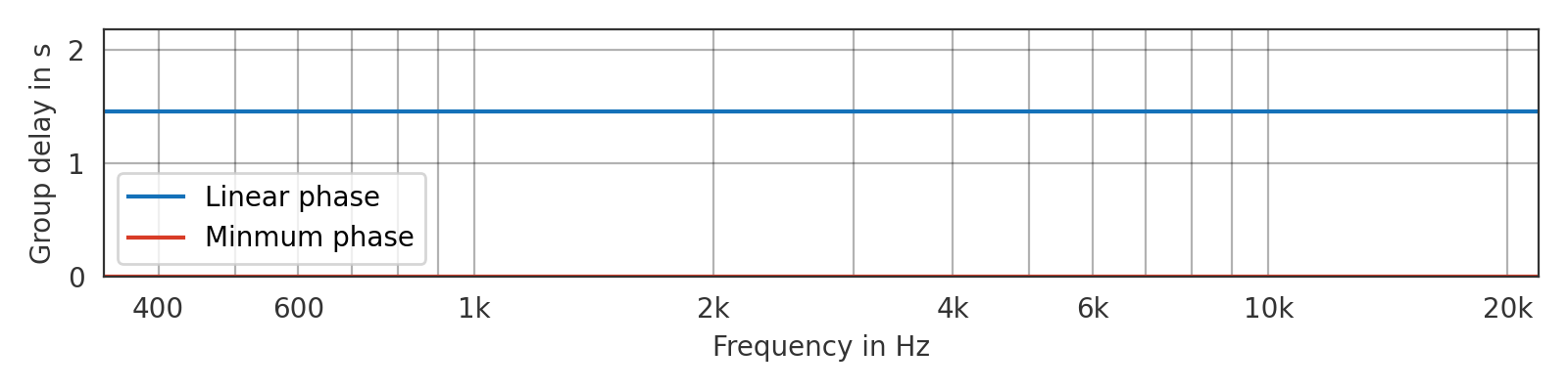
Minmum-phase version of an ideal impulse with a group delay of 64 samples

>>> import pyfar as pf
>>> import matplotlib.pyplot as plt
>>> # create linear and minimum phase signal
>>> impulse_linear_phase = pf.signals.impulse(129, delay=64)
>>> impulse_minmum_phase = pf.dsp.minimum_phase(
...     impulse_linear_phase, method='homomorphic')
>>> # plot the group delay
>>> plt.figure(figsize=(8, 2))
>>> pf.plot.group_delay(impulse_linear_phase, label='Linear phase')
>>> pf.plot.group_delay(impulse_minmum_phase, label='Minmum phase')
>>> plt.legend()

(Source code, png, hires.png, pdf)

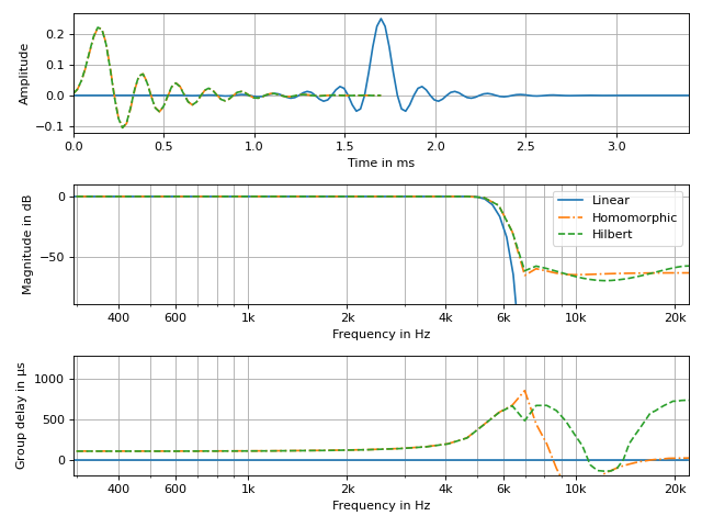
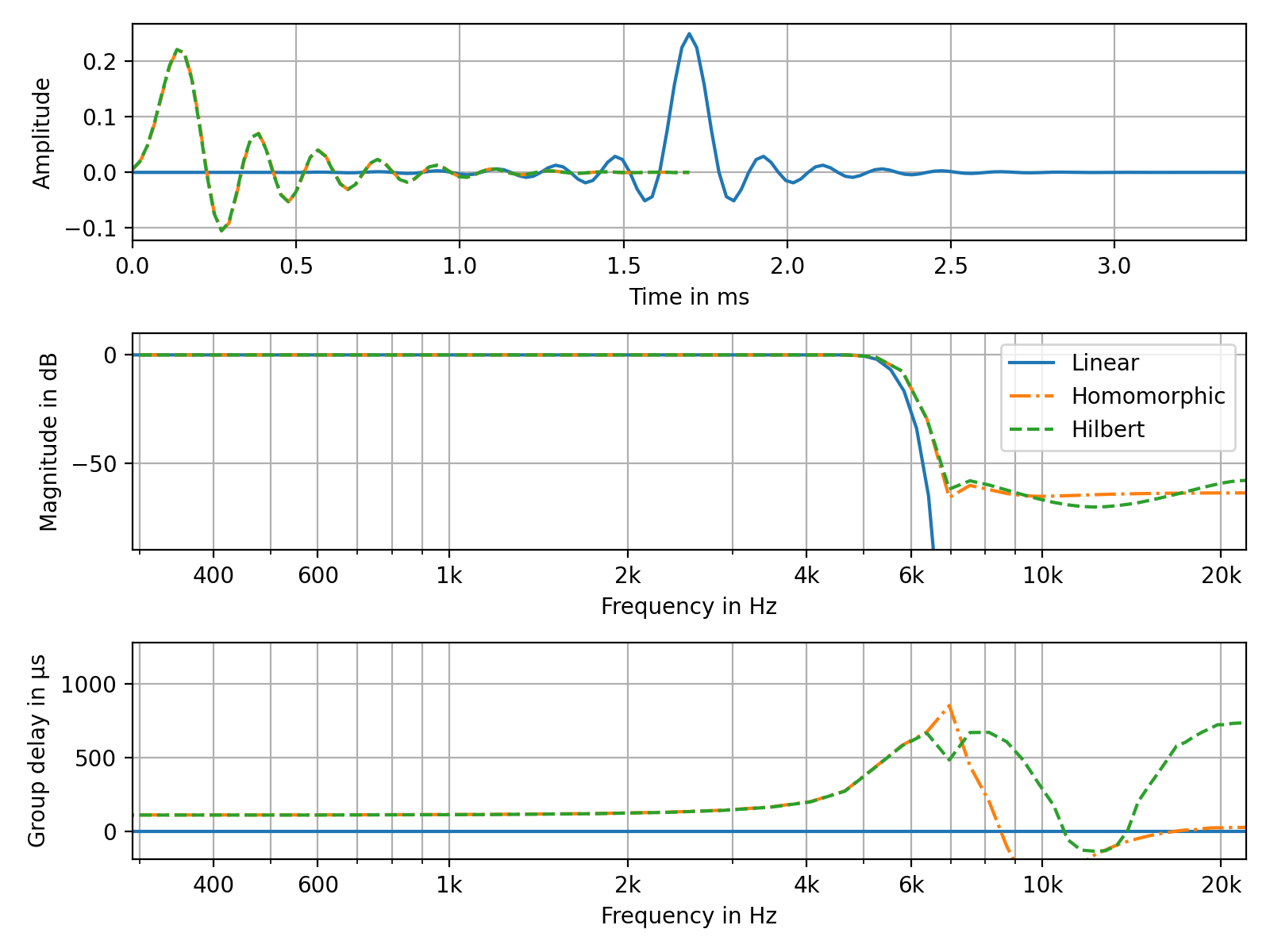
Create a minimum phase equivalent of a linear phase FIR low-pass filter

>>> import pyfar as pf
>>> import numpy as np
>>> from scipy.signal import remez
>>> import matplotlib.pyplot as plt
>>> # create minimum phase signals with different methods
>>> freq = [0, 0.2, 0.3, 1.0]
>>> desired = [1, 0]
>>> h_linear = pf.Signal(remez(151, freq, desired, Hz=2.), 44100)
>>> h_min_hom = pf.dsp.minimum_phase(h_linear, method='homomorphic')
>>> h_min_hil = pf.dsp.minimum_phase(h_linear, method='hilbert')
>>> # plot the results
>>> fig, axs = plt.subplots(3, figsize=(8, 6))
>>> for h, style in zip(
...         (h_linear, h_min_hom, h_min_hil),
...         ('-', '-.', '--')):
>>>     pf.plot.time(h, linestyle=style, ax=axs[0])
>>>     axs[0].grid(True)
>>>     pf.plot.freq(h, linestyle=style, ax=axs[1])
>>>     pf.plot.group_delay(h, linestyle=style, ax=axs[2])
>>> axs[1].legend(['Linear', 'Homomorphic', 'Hilbert'])

(Source code, png, hires.png, pdf)

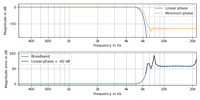
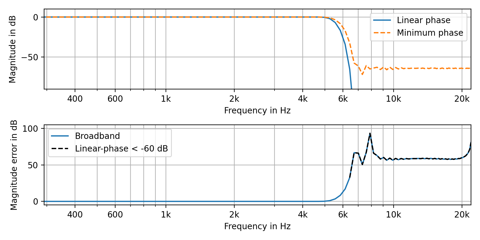
Return the magnitude ratios between the minimum and linear phase filters and indicate frequencies where the linear phase filter exhibits small amplitudes.

>>> import pyfar as pf
>>> import numpy as np
>>> from scipy.signal import remez
>>> import matplotlib.pyplot as plt
>>> # generate linear and minimum phase signal
>>> freq = [0, 0.2, 0.3, 1.0]
>>> desired = [1, 0]
>>> h_linear = pf.Signal(remez(151, freq, desired, Hz=2.), 44100)
>>> h_minimum, ratio = pf.dsp.minimum_phase(h_linear,
...     method='homomorphic', return_magnitude_ratio=True)
>>> # plot signals and difference between them
>>> fig, axs = plt.subplots(2, figsize=(8, 4))
>>> pf.plot.freq(h_linear, linestyle='-', ax=axs[0])
>>> pf.plot.freq(h_minimum, linestyle='--', ax=axs[0])
>>> pf.plot.freq(ratio, linestyle='-', ax=axs[1])
>>> mask = np.abs(h_linear.freq) < 10**(-60/20)
>>> ratio_masked = pf.FrequencyData(
...     ratio.freq[mask], ratio.frequencies[mask[0]])
>>> pf.plot.freq(ratio_masked, color='k', linestyle='--', ax=axs[1])
>>> axs[1].set_ylabel('Magnitude error in dB')
>>> axs[0].legend(['Linear phase', 'Minimum phase'])
>>> axs[1].legend(['Broadband', 'Linear-phase < -60 dB'])
>>> axs[1].set_ylim((-5, 105))

(Source code, png, hires.png, pdf)

pyfar.dsp.pad_zeros(signal, pad_width, mode='after')[source]¶

Pad a signal with zeros in the time domain.

Parameters

signal (Signal) – The signal which is to be extended.
pad_width (int) – The number of samples to be padded.
mode (str, optional) –
The padding mode:

'after'
Append zeros to the end of the signal

'before'
Pre-pend zeros before the starting time of the signal

'center'
Insert the number of zeros in the middle of the signal. This mode can be used to pad signals with a symmetry with respect to the time t=0.

The default is 'after'.

Returns

The zero-padded signal.

Return type

Signal

Examples

>>> import pyfar as pf
>>> impulse = pf.signals.impulse(512, amplitude=1)
>>> impulse_padded = pf.dsp.pad_zeros(impulse, 128, mode='after')

pyfar.dsp.phase(signal, deg=False, unwrap=False)[source]¶

Returns the phase for a given signal object.

Parameters

signal (Signal, FrequencyData) – pyfar Signal or FrequencyData object.
deg (Boolean) – Specifies, whether the phase is returned in degrees or radians.
unwrap (Boolean) – Specifies, whether the phase is unwrapped or not. If set to '360', the phase is wrapped to 2 pi.

Returns

phase – The phase of the signal.

Return type

numpy array

pyfar.dsp.regularized_spectrum_inversion(signal, freq_range, regu_outside=1.0, regu_inside=1e-10, regu_final=None, normalized=True)[source]¶

Invert the spectrum of a signal applying frequency dependent regularization.

Regularization can either be specified within a given frequency range using two different regularization factors, or for each frequency individually using the parameter regu_final. In the first case the regularization factors for the frequency regions are cross-faded using a raised cosine window function with a width of $\sqrt{2}f$ above and below the given frequency range. Note that the resulting regularization function is adjusted to the quadratic maximum of the given signal. In case the regu_final parameter is used, all remaining options are ignored and an array matching the number of frequency bins of the signal needs to be given. In this case, no normalization of the regularization function is applied.

Finally, the inverse spectrum is calculated as 4, 5,

$S^{-1}(f) = \frac{S^*(f)}{S^*(f)S(f) + \epsilon(f)}$

Parameters

signal (Signal) – The signals which spectra are to be inverted.
freq_range (tuple, array_like, double) – The upper and lower frequency limits outside of which the regularization factor is to be applied.
regu_outside (float, optional) – The normalized regularization factor outside the frequency range. The default is 1.
regu_inside (float, optional) – The normalized regularization factor inside the frequency range. The default is 10**(-200/20) (-200 dB).
regu_final (float, array_like, optional) – The final regularization factor for each frequency, default None. If this parameter is set, the remaining regularization factors are ignored.
normalized (bool) – Flag to indicate if the normalized spectrum (according to signal.fft_norm) should be inverted. The default is True.

Returns

The resulting signal after inversion.

Return type

Signal

References

4: O. Kirkeby and P. A. Nelson, “Digital Filter Design for Inversion Problems in Sound Reproduction,” J. Audio Eng. Soc., vol. 47, no. 7, p. 13, 1999.
5: P. C. Hansen, Rank-deficient and discrete ill-posed problems: numerical aspects of linear inversion. Philadelphia: SIAM, 1998.

pyfar.dsp.spectrogram(signal, window='hann', window_length=1024, window_overlap_fct=0.5, normalize=True)[source]¶

Compute the magnitude spectrum versus time.

This is a wrapper for scipy.signal.spectogram with two differences. First, the returned times refer to the start of the FFT blocks, i.e., the first time is always 0 whereas it is window_length/2 in scipy. Second, the returned spectrogram is normalized according to signal.fft_norm if the normalize parameter is set to True.

Parameters

signal (Signal) – Signal to compute spectrogram of.
window (str) – Specifies the window (see scipy.signal.windows). The default is 'hann'.
window_length (integer) – Window length in samples, the default ist 1024.
window_overlap_fct (double) – Ratio of points to overlap between FFT segments [0…1]. The default is 0.5.
normalize (bool) – Flag to indicate if the FFT normalization should be applied to the spectrogram according to signal.fft_norm. The default is True.

Returns

frequencies (numpy array) – Frequencies in Hz at which the magnitude spectrum was computed
times (numpy array) – Times in seconds at which the magnitude spectrum was computed
spectrogram (numpy array)

pyfar.dsp.time_shift(signal, shift, unit='samples')[source]¶

Apply a time-shift to a signal.

The shift is performed as a cyclic shift on the time axis, potentially resulting in non-causal signals for negative shift values.

Parameters

signal (Signal) – The signal to be shifted
shift (int, float) – The time-shift value. A positive value will result in right shift on the time axis (delaying of the signal), whereas a negative value yields a left shift on the time axis (non-causal shift to a earlier time). If a single value is given, the same time shift will be applied to each channel of the signal. Individual time shifts for each channel can be performed by passing an array matching the signals channel dimensions cshape.
unit (str, optional) – Unit of the shift variable, this can be either 'samples' or 's' for seconds. By default 'samples' is used. Note that in the case of specifying the shift time in seconds, the value is rounded to the next integer sample value to perform the shift.

Returns

The time-shifted signal.

Return type

Signal

Examples

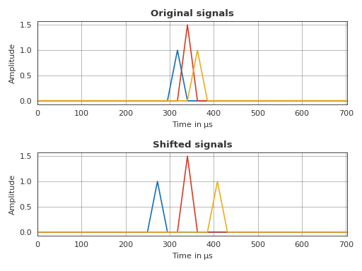
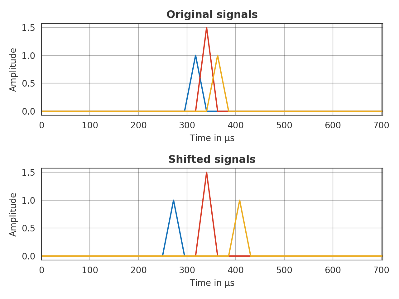
Individually shift a set of ideal impulses stored in three different channels and plot the resulting signals

>>> import pyfar as pf
>>> import matplotlib.pyplot as plt
>>> # generate and shift the impulses
>>> impulse = pf.signals.impulse(
...     32, amplitude=(1, 1.5, 1), delay=(14, 15, 16))
>>> shifted = pf.dsp.time_shift(impulse, [-2, 0, 2])
>>> # time domain plot
>>> pf.plot.use('light')
>>> _, axs = plt.subplots(2, 1)
>>> pf.plot.time(impulse, ax=axs[0])
>>> pf.plot.time(shifted, ax=axs[1])
>>> axs[0].set_title('Original signals')
>>> axs[1].set_title('Shifted signals')
>>> plt.tight_layout()

(Source code, png, hires.png, pdf)

pyfar.dsp.time_window(signal, interval, window='hann', shape='symmetric', unit='samples', crop='none', return_window=False)[source]¶

Apply time window to signal.

This function uses the windows implemented in scipy.signal.windows.

Parameters

signal (Signal) – Signal object to be windowed.
interval (array_like) – If interval has two entries, these specify the beginning and the end of the symmetric window or the fade-in / fade-out (see parameter shape). If interval has four entries, a window with fade-in between the first two entries and a fade-out between the last two is created, while it is constant in between (ignores shape). The unit of interval is specified by the parameter unit. See below for more details.
window (string, float, or tuple, optional) – The type of the window. See below for a list of implemented windows. The default is 'hann'.
shape (string, optional) –

'symmetric'
General symmetric window, the two values in interval define the first and last samples of the window.

'symmetric_zero'
Symmetric window with respect to t=0, the two values in interval define the first and last samples of fade-out. crop is ignored.

'left'
Fade-in, the beginning and the end of the fade is defined by the two values in interval. See Notes for more details.

'right'
Fade-out, the beginning and the end of the fade is defined by the two values in interval. See Notes for more details.

The default is 'symmetric'.
unit (string, optional) – Unit of interval. Can be set to 'samples' or 's' (seconds). Time values are rounded to the nearest sample. The default is 'samples'.
crop (string, optional) –

'none'
The length of the windowed signal stays the same.

'window'
The signal is truncated to the windowed part.

'end'
Only the zeros at the end of the windowed signal are cropped, so the original phase is preserved.

The default is 'none'.
return_window (bool, optional) – If True, both the windowed signal and the time window are returned. The default is False.

Returns

signal_windowed (Signal) – Windowed signal object
window (Signal) – Time window used to create the windowed signal, only returned if return_window=True.

Notes

For a fade-in, the indexes of the samples given in interval denote the first sample of the window which is non-zero and the first which is one. For a fade-out, the samples given in interval denote the last sample which is one and the last which is non-zero.

This function calls scipy.signal.windows.get_window to create the window. Available window types:

boxcar
triang
blackman
hamming
hann
bartlett
flattop
parzen
bohman
blackmanharris
nuttall
barthann
kaiser (needs beta, see kaiser_window_beta)
gaussian (needs standard deviation)
general_gaussian (needs power, width)
dpss (needs normalized half-bandwidth)
chebwin (needs attenuation)
exponential (needs center, decay scale)
tukey (needs taper fraction)
taylor (needs number of constant sidelobes, sidelobe level)

If the window requires no parameters, then window can be a string. If the window requires parameters, then window must be a tuple with the first argument the string name of the window, and the next arguments the needed parameters.

Examples

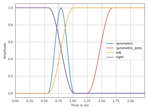
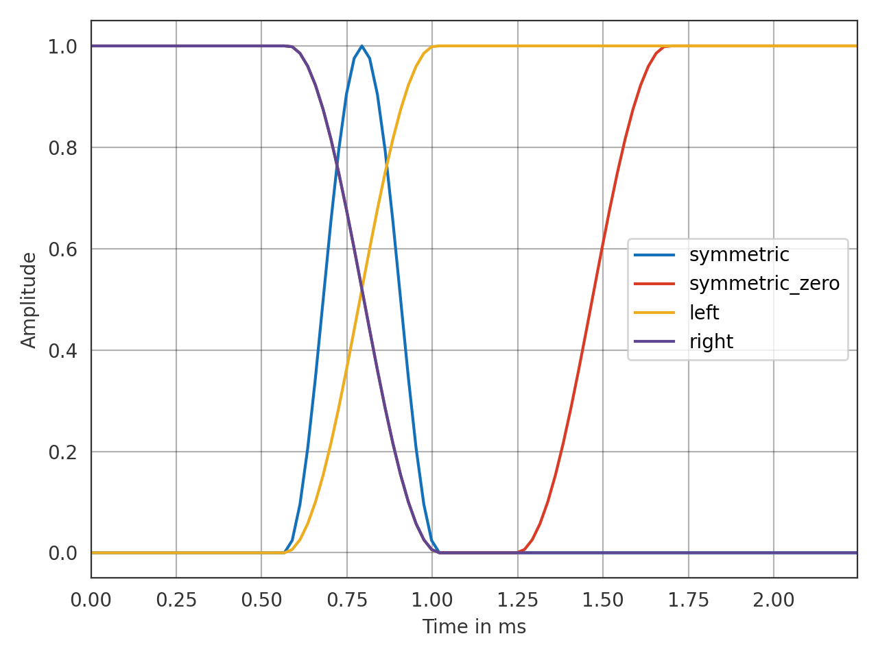
Options for parameter shape.

>>> import pyfar as pf
>>> import numpy as np
>>> signal = pf.Signal(np.ones(100), 44100)
>>> for shape in ['symmetric', 'symmetric_zero', 'left', 'right']:
>>>     signal_windowed = pf.dsp.time_window(
...         signal, interval=[25,45], shape=shape)
>>>     ax = pf.plot.time(signal_windowed, label=shape)
>>> ax.legend(loc='right')

(Source code, png, hires.png, pdf)

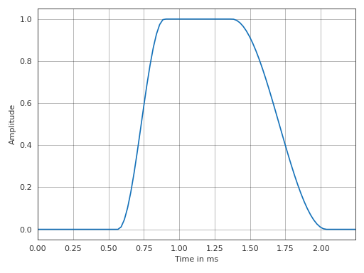
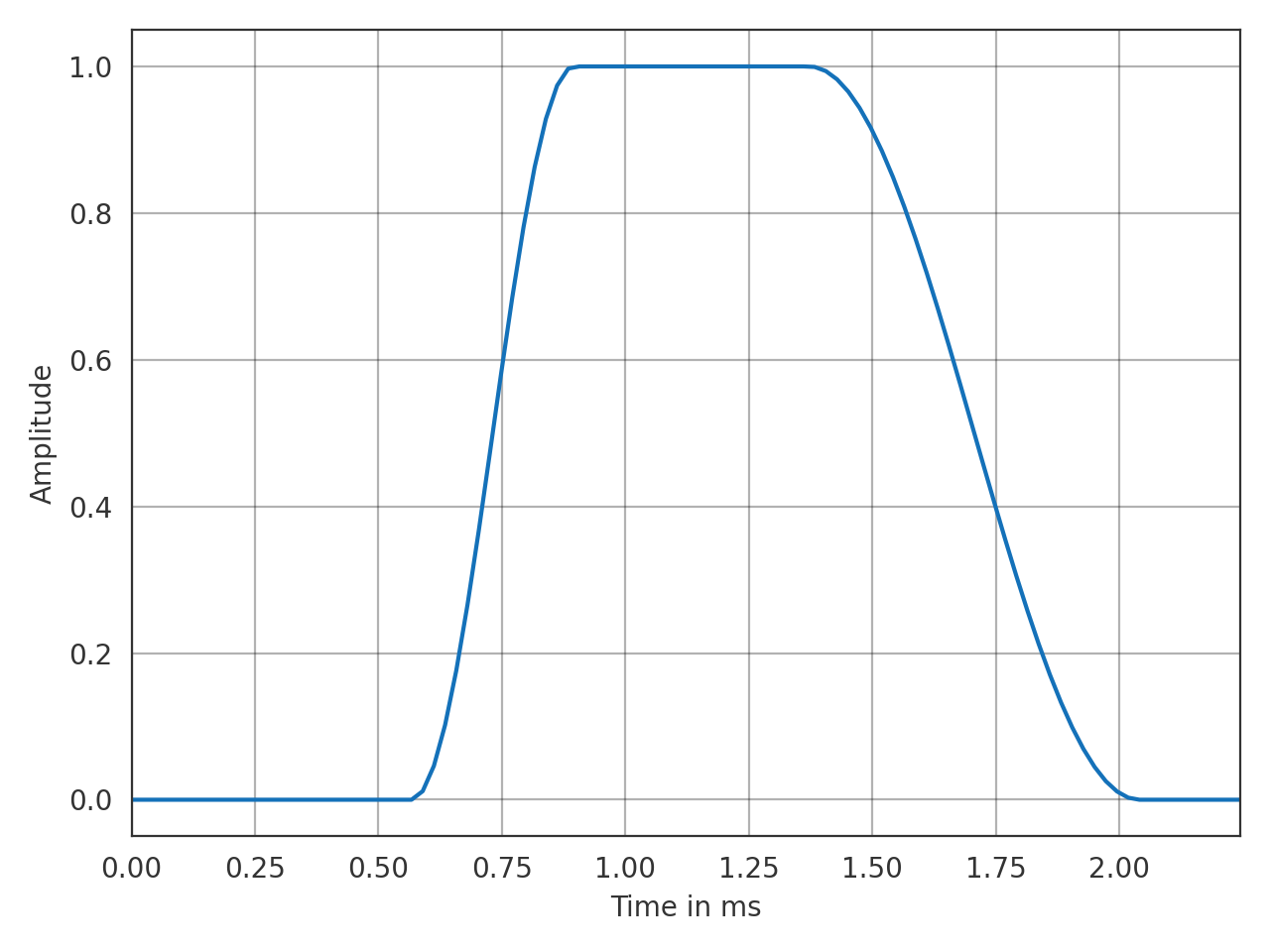
Window with fade-in and fade-out defined by four values in interval.

>>> import pyfar as pf
>>> import numpy as np
>>> signal = pf.Signal(np.ones(100), 44100)
>>> signal_windowed = pf.dsp.time_window(
...         signal, interval=[25, 40, 60, 90], window='hann')
>>> pf.plot.time(signal_windowed)