
pyfar.dsp.filter#
The following documents the pyfar filters. Visit the Overview of filters for an overview of the different filters and the Filtering pyfar Signals for more information on using pyfar filter objects.
Classes:
|
Generate reconstructing auditory filter bank. |
Functions:
|
Create and apply first or second order allpass filter. |
|
Create and apply second order bell (parametric equalizer) filter. |
|
Create and apply digital Bessel/Thomson IIR filter. |
|
Create and apply a digital Butterworth IIR filter. |
|
Create and apply digital Chebyshev Type I IIR filter. |
|
Create and apply digital Chebyshev Type II IIR filter. |
Check magnitude tolerance of fractional octave band filters. |
|
|
Create and apply Linkwitz-Riley crossover network. |
|
Create and apply digital Elliptic (Cauer) IIR filter. |
|
Get frequencies that are linearly spaced on the ERB frequency scale. |
|
Create and/or apply an energy preserving fractional octave filter bank. |
Return the octave center frequencies according to the IEC 61260:1:2014 standard. |
|
|
Create and apply an A or C weighting filter. |
|
Create and/or apply first or second order high shelf filter. |
|
Create and apply constant slope filter from cascaded 2nd order high shelves. |
|
|
|
|
|
Create and apply first or second order low shelf filter. |
|
Create and apply constant slope filter from cascaded 2nd order low shelves. |
|
|
|
|
|
Create and apply or return a second order IIR notch filter. |
Create and/or apply an amplitude preserving fractional octave filter bank. |
- class pyfar.dsp.filter.GammatoneBands(frequency_range, resolution=1, reference_frequency=1000, delay=0.004, sampling_rate=44100)[source]#
Bases:
objectGenerate reconstructing auditory filter bank.
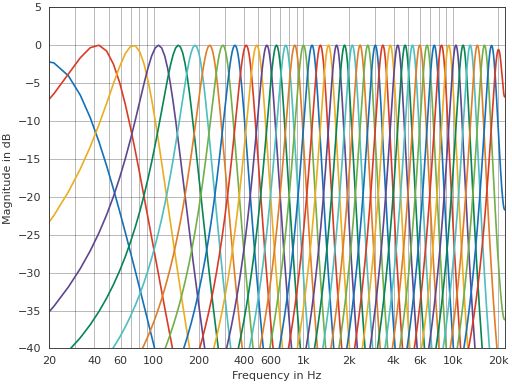
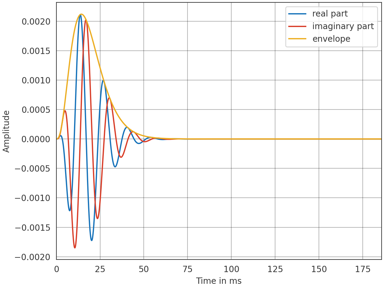
Generate a forth order reconstructing Gammatone auditory filter bank according to [1]. The center frequencies of the Gammatone filters are calculated using the ERB scale (see
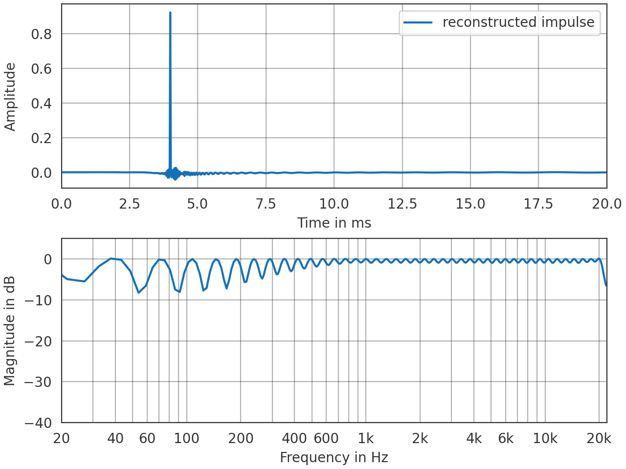
erb_frequencies).This is a Python port of the hohmann2002 filter bank contained in the Auditory Modeling Toolbox [2]. The filter bank can handle single and multi channel input and allows for an almost perfect reconstruction of the input signal (see examples below).
Calling
GFB = GammatoneBands()constructs the filter bank. Afterwards the class methodsGFB.process()andGFB.reconstruct()can be used to filter and reconstruct signals. All relevant data such as the filter coefficients can be obtained for example throughGFB.coefficients. See below for more documentation.- Parameters:
frequency_range (array_like) – The upper and lower frequency in Hz between which the filter bank is constructed. Values must be larger than 0 and not exceed half the sampling rate.
resolution (number) – The frequency resolution of the filter bands in equivalent rectangular bandwidth (ERB) units. The bands of the filter bank are distributed linearly on the ERB scale. The default value of
1results in one filter band per ERB. A value of0.5would result in two filter bands per ERB.reference_frequency (number) – The frequency relative to which the filter bands are distributed. The default is
1000Hz.delay (number) – The delay in seconds that the filter bank will have, i.e., the delay that is added to the input signal after being filtered and summed again. The default is
0.004seconds.sampling_rate (number) – The sampling rate of the filter bank in Hz. The default is
44100Hz.
Examples
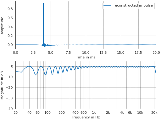
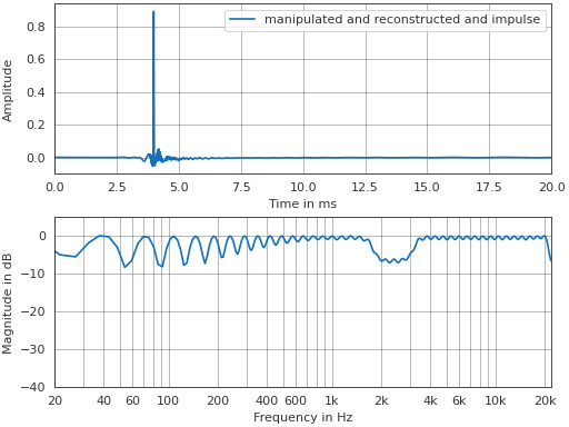
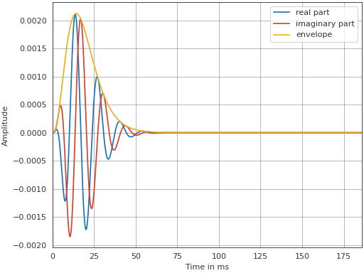
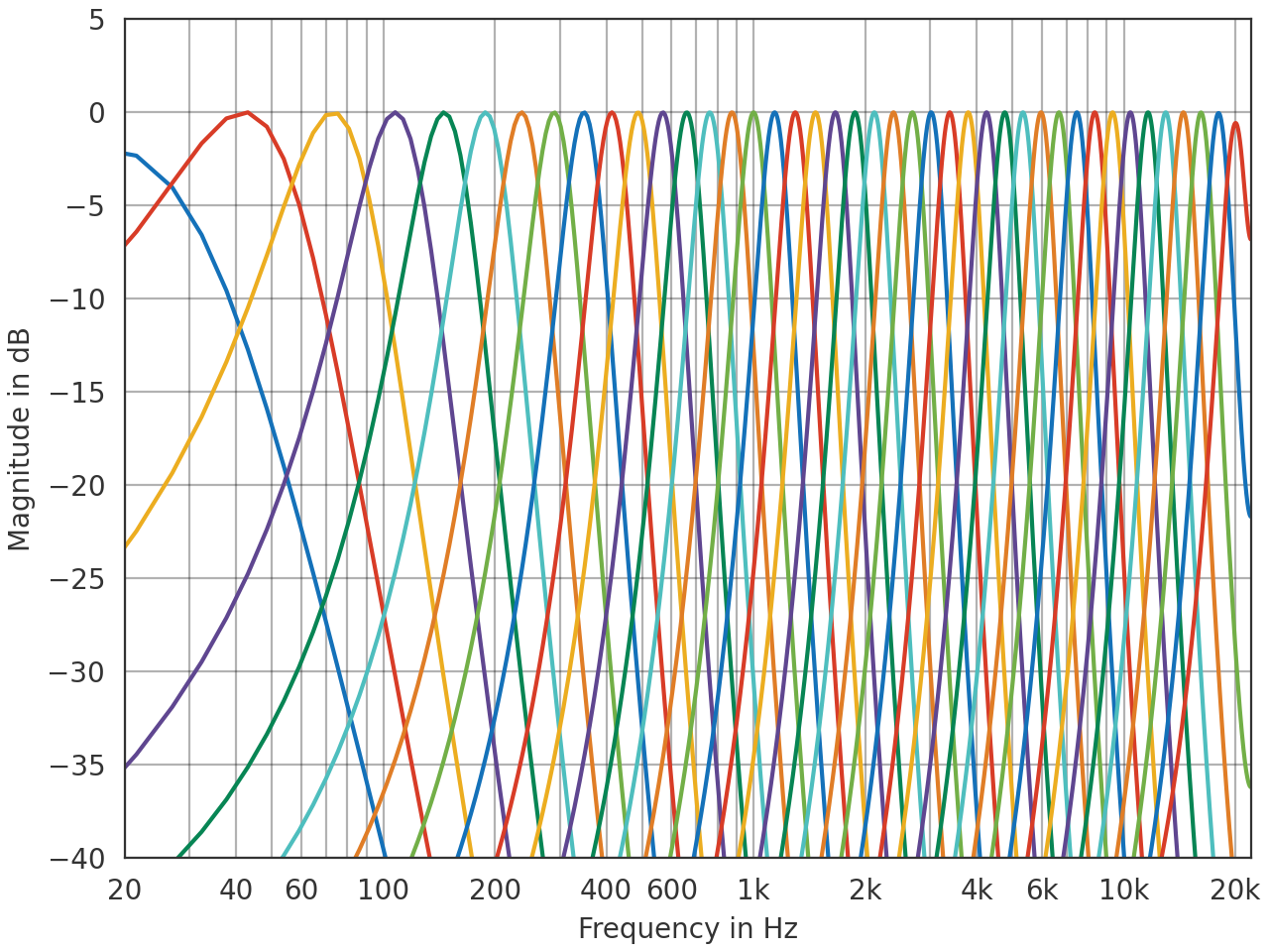
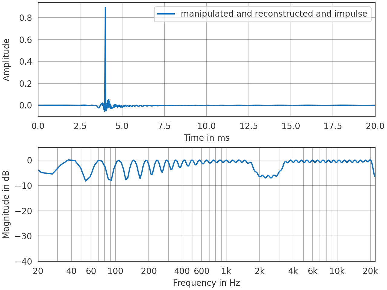
>>> import pyfar as pf
>>> import numpy as np
>>> import matplotlib.pyplot as plt
>>>
>>> # generate the filter bank object
>>> GFB = pf.dsp.filter.GammatoneBands([0, 22050])
>>>
>>> # apply the filter bank to an impulse
>>> x = pf.signals.impulse(2**13)
>>> real, imag = GFB.process(x)
>>> env = pf.Signal(np.abs(real.time + 1j * imag.time), 44100)
>>>
>>> # use pyfar plot style
>>> pf.plot.use()
>>>
>>> # the output is complex:
>>> # Real part gives band-limited Gammatone output
>>> # Imaginary part gives the Hilbert Transform thereof
>>> # Absolute value gives the Envelope
>>> plt.figure()
>>> ax = pf.plot.time(real[2], label='real part', unit='ms')
>>> pf.plot.time(imag[2], label='imaginary part', unit='ms')
>>> pf.plot.time(env[2], label='envelope', unit='ms')
>>> plt.legend()
>>>
>>> # show the magnitude response of the filter bank
>>> plt.figure()
>>> ax = pf.plot.freq(real)
>>> ax.set_ylim(-40, 5)
>>>
>>> # reconstruct the filtered impulse
>>> # the reconstruction error can be decreased
>>> # using the filter bank parameter 'resolution'
>>> y = GFB.reconstruct(real, imag)
>>> plt.figure()
>>> ax = pf.plot.time_freq(y, label="reconstructed impulse", unit='ms')
>>> ax[0].set_xlim(0, 20)
>>> ax[1].set_ylim(-40, 5)
>>> ax[0].legend()
>>>
>>> # manipulate filter output before the reconstruction
>>> # (manipulations must be applied to the real and imaginary output)
>>> real.time[20:25] *= .5
>>> imag.time[20:25] *= .5
>>>
>>> y = GFB.reconstruct(real, imag)
>>> plt.figure()
>>> ax = pf.plot.time_freq(
...     y, unit='ms',
...     label="manipulated and reconstructed and impulse")
>>> ax[0].set_xlim(0, 20)
>>> ax[1].set_ylim(-40, 5)
>>> ax[0].legend()

References
Attributes:
Get the filter coefficients a as in Eq.
Get the desired delay of the filter bank in seconds.
Get the delays required for summing the filter bands.
Get the center frequencies of the Gammatone filters in Hz.
Get the frequency range of the filter bank in Hz.
Get the gains required for summing the filter bands.
Get the number of bands in the filter bank.
Get the normalization per band described below Eq.
Get the phase factors required for summing the filter bands.
Get the reference frequency of the filter bank in Hz.
Get the resolution of the filter bank in ERB units.
Get the sampling rate of the filter bank in Hz.
Methods:
copy()Return a copy of the audio object.
impulse_response([n_samples])Compute the impulse response of the gammatone filterbank.
minimum_impulse_response_length([unit, ...])Estimate the minimum length of the filterbank's impulse response.
process(signal[, reset])Filter an input signal.
reconstruct(real, imag)Reconstruct filter bands.
- property coefficients#
Get the filter coefficients a as in Eq. (7) in Hohmann 2002 per band.
- property delay#
Get the desired delay of the filter bank in seconds.
- property delays#
Get the delays required for summing the filter bands.
Section 4 in Hohmann 2002 describes, how the delays are calculated.
- property frequencies#
Get the center frequencies of the Gammatone filters in Hz.
- property frequency_range#
Get the frequency range of the filter bank in Hz.
- property gains#
Get the gains required for summing the filter bands.
Section 4 in Hohmann 2002 describes, how the gains are calculated.
- impulse_response(n_samples=None)[source]#
Compute the impulse response of the gammatone filterbank.
- Parameters:
n_samples (int, optional) – Length in samples for which the impulse response is computed. The default is
Nonein which casen_samplesis computed as the maximum value across filter channels returned byminimum_impulse_response_length. A warning is returned ifn_samplesis shorter than the maximum value returned byminimum_impulse_response_length.- Returns:
impulse_response_real (Signal) – The impulse response of the real part of the filterbank of
cshape = (:py:func:`~n_bands`, ).impulse_response_imag (Signal) – The impulse response of the imaginary part of the filterbank of
cshape = (:py:func:`~n_bands`, ).
- minimum_impulse_response_length(unit='samples', tolerance=5e-05)[source]#
Estimate the minimum length of the filterbank’s impulse response.
The length is estimated using
FilterSOS.minimum_impulse_response_length.- Parameters:
unit (string, optional) – The unit in which the length is returned. Can be
'samples'or's'(seconds). The default is'samples'.tolerance (float, optional) – Tolerance for the accuracy. Smaller tolerances will result in larger impulse response lengths. The default is
5e-5.
- Returns:
minimum_impulse_response_length – An integer array of
shape = (n_bands, )containing the length in specified unit with the number of gammatone-bandsn_bands.- Return type:
array
- property n_bands#
Get the number of bands in the filter bank.
- property normalizations#
Get the normalization per band described below Eq. (9) in Hohmann 2002.
- property phase_factors#
Get the phase factors required for summing the filter bands.
Section 4 in Hohmann 2002 describes, how the factors are calculated.
- process(signal, reset=True)[source]#
Filter an input signal.
The filter output is a complex valued time signal, whose real and imaginary part are returned separately.
If the filter bank is used for analysis purposes only, the imaginary part is not required for further processing.
If the filter bank is used for analysis and re-synthesis, any further processing must be applied to the real and imaginary part. Any complex-valued operations must be applied to the complex valued output as a whole.
- Parameters:
signal (Signal) – The data to be filtered
reset (bool, optional) – If true the internal state of the filter bank is reset before the filters are applied. Not resetting the state can be useful for blockwise processing. The default is
True.
- Returns:
real (Signal) – The real part of the complex output signal. This represents the band-limited Gammatone filter output.
imag (Signal) – The imaginary part of the complex output signal. This approximates the Hilbert transform of the band-limited Gammatone filter output.
Notes
sqrt(real.time**2 + imag.time**2)gives the envelope of the Gammatone filter output.If the cshape of the output signals
real.cshapeandimag.cshapegenerally is(self.n_bands, ) + signal.cshape.An exception to this occurs if
signal.cshapeis(1, ), i.e., signal is a single channel signal. In this case the cshape of the output signals is(self.n_bands)and not(self.n_bands, 1).
- reconstruct(real, imag)[source]#
Reconstruct filter bands.
The summation process is described in Section 4 of Hohmann 2002 and uses the pre-calculated delays, phase factors and gains.
- Parameters:
- Returns:
reconstructed – The summed input.
summed.cshapematches thecshapeor the original signal before it was filtered.- Return type:
- property reference_frequency#
Get the reference frequency of the filter bank in Hz.
- property resolution#
Get the resolution of the filter bank in ERB units.
- property sampling_rate#
Get the sampling rate of the filter bank in Hz.
- pyfar.dsp.filter.allpass(signal, frequency, order, coefficients=None, sampling_rate=None)[source]#
Create and apply first or second order allpass filter.
Allpass filters have an almost constant group delay below their cut-off frequency and are often used in analogue loudspeaker design. The filter transfer function is based on Tietze et al. [3]:
\[A(s) = \frac{1-\frac{a_i}{\omega_c} s+\frac{b_i} {\omega_c^2} s^2}{1+\frac{a_i}{\omega_c} s +\frac{b_i}{\omega_c^2} s^2},\]where \(\omega_c = 2 \pi f_c\) with the cut-off frequency \(f_c\) and \(s=\mathrm{i} \omega\).
By definition the
bicoefficient of a first order allpass is0.Uses the implementation of [4].
- Parameters:
signal (Signal, None) – The signal to be filtered. Pass
Noneto create the filter without applying it.frequency (number) – Cutoff frequency of the allpass in Hz.
order (number) – Order of the allpass filter. Must be
1or2.coefficients (number, list, optional) –
Filter characteristic coefficients
biandai.For 1st order allpass provide ai-coefficient as single value.n The default is
ai = 0.6436.For 2nd order allpass provide coefficients as list
[bi, ai].n The default isbi = 0.8832,ai = 1.6278.
Defaults are chosen according to Tietze et al. (Fig. 12.66) for maximum flat group delay.
sampling_rate (None, number) – The sampling rate in Hz. Only required if signal is
None. The default isNone.
- Returns:
signal (Signal) – The filtered signal. Only returned if
sampling_rate = None.filter (FilterIIR) – Filter object. Only returned if
signal = None.
References
Examples
First and second order allpass filter with
fc = 1000Hz.import pyfar as pf import matplotlib.pyplot as plt # impulse to be filtered impulse = pf.signals.impulse(256) orders = [1, 2] labels = ['First order', 'Second order'] fig, (ax1, ax2) = plt.subplots(2,1, layout='constrained') for (order, label) in zip(orders, labels): # create and apply allpass filter sig_filt = pf.dsp.filter.allpass(impulse, 1000, order) pf.plot.group_delay(sig_filt, unit='samples', label=label, ax=ax1) pf.plot.phase(sig_filt, label=label, ax=ax2, unwrap = True) ax1.set_title('1. and 2. order allpass filter with fc = 1000 Hz') ax2.legend()
(
Source code,png,hires.png,pdf)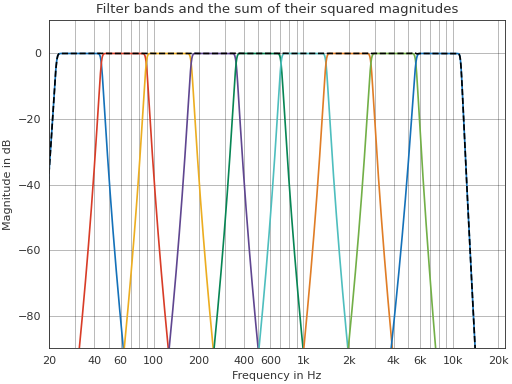
- pyfar.dsp.filter.bell(signal, center_frequency, gain, quality, bell_type='II', quality_warp='cos', sampling_rate=None)[source]#
Create and apply second order bell (parametric equalizer) filter.
Uses the implementation of [5].
- Parameters:
signal (Signal, None) – The signal to be filtered. Pass
Noneto create the filter without applying it.center_frequency (number) – Center frequency of the parametric equalizer in Hz
gain (number) – Gain of the parametric equalizer in dB
quality (number) – Quality of the parametric equalizer, i.e., the inverse of the bandwidth
bell_type (str) –
Defines the bandwidth/quality. The default is
'II'.'I'not recommended. Also known as ‘constant Q’.
'II'defines the bandwidth by the points 3 dB below the maximum if the gain is positive and 3 dB above the minimum if the gain is negative. Also known as ‘symmetric’.
'III'defines the bandwidth by the points at gain/2. Also known as ‘half pad loss’.
quality_warp (str) – Sets the pre-warping for the quality (
'cos','sin', or'tan'). The default is'cos'.sampling_rate (None, number) – The sampling rate in Hz. Only required if signal is
None. The default isNone.
- Returns:
signal (Signal) – The filtered signal. Only returned if
sampling_rate = None.filter (FilterIIR) – Filter object. Only returned if
signal = None.
References
- pyfar.dsp.filter.bessel(signal, N, frequency, btype='lowpass', norm='phase', sampling_rate=None)[source]#
Create and apply digital Bessel/Thomson IIR filter.
This is a wrapper for
scipy.signal.bessel. Which creates digital Bessel filter coefficients in second-order sections (SOS).- Parameters:
signal (Signal, None) – The Signal to be filtered. Pass
Noneto create the filter without applying it.N (int) – The order of the Bessel/Thomson filter.
frequency (number, array like) – The cut off-frequency in Hz if btype is
'lowpass'or'highpass'. An array like containing the lower and upper cut-off frequencies in Hz if btype is bandpass or bandstop.btype (str) – One of the following
'lowpass','highpass','bandpass','bandstop'. The default is'lowpass'.norm (str) –
Critical frequency normalization:
'phase'The filter is normalized such that the phase response reaches its midpoint at angular (e.g. rad/s) frequency Wn. This happens for both low-pass and high-pass filters, so this is the “phase-matched” case. The magnitude response asymptotes are the same as a Butterworth filter of the same order with a cutoff of Wn. This is the default, and matches MATLAB’s implementation.
'delay'The filter is normalized such that the group delay in the passband is 1/Wn (e.g., seconds). This is the “natural” type obtained by solving Bessel polynomials.
'mag'The filter is normalized such that the gain magnitude is -3 dB at the angular frequency Wn.
The default is ‘phase’.
sampling_rate (None, number) – The sampling rate in Hz. Only required if signal is None. The default is None.
- Returns:
signal (Signal) – The filtered signal. Only returned if
sampling_rate = None.filter (FilterSOS) – SOS Filter object. Only returned if
signal = None.
- pyfar.dsp.filter.butterworth(signal, N, frequency, btype='lowpass', sampling_rate=None)[source]#
Create and apply a digital Butterworth IIR filter.
This is a wrapper for
scipy.signal.butter. Which creates digital Butterworth filter coefficients in second-order sections (SOS).- Parameters:
signal (Signal, None) – The Signal to be filtered. Pass
Noneto create the filter without applying it.N (int) – The order of the Butterworth filter
frequency (number, array like) – The cut off-frequency in Hz if btype is lowpass or highpass. An array like containing the lower and upper cut-off frequencies in Hz if btype is bandpass or bandstop.
btype (str) – One of the following
'lowpass','highpass','bandpass','bandstop'. The default is'lowpass'.sampling_rate (None, number) – The sampling rate in Hz. Only required if signal is
None. The default isNone.
- Returns:
signal (Signal) – The filtered signal. Only returned if
sampling_rate = None.filter (FilterSOS) – SOS Filter object. Only returned if
signal = None.
- pyfar.dsp.filter.chebyshev1(signal, N, ripple, frequency, btype='lowpass', sampling_rate=None)[source]#
Create and apply digital Chebyshev Type I IIR filter.
This is a wrapper for
scipy.signal.cheby1. Which creates digital Chebyshev Type I filter coefficients in second-order sections (SOS).- Parameters:
signal (Signal, None) – The Signal to be filtered. Pass
Noneto create the filter without applying it.N (int) – The order of the Chebychev filter.
ripple (number) – The passband ripple in dB.
frequency (number, array like) – The cut off-frequency in Hz if btype is
'lowpass'or'highpass'. An array like containing the lower and upper cut-off frequencies in Hz if btype is'bandpass'or'bandstop'.btype (str) – One of the following
'lowpass','highpass','bandpass','bandstop'. The default is'lowpass'.sampling_rate (None, number) – The sampling rate in Hz. Only required if signal is
None. The default isNone.
- Returns:
signal (Signal) – The filtered signal. Only returned if
sampling_rate = None.filter (FilterSOS) – SOS Filter object. Only returned if
signal = None.
- pyfar.dsp.filter.chebyshev2(signal, N, attenuation, frequency, btype='lowpass', sampling_rate=None)[source]#
Create and apply digital Chebyshev Type II IIR filter.
This is a wrapper for
scipy.signal.cheby2. Which creates digital Chebyshev Type II filter coefficients in second-order sections (SOS).- Parameters:
signal (Signal, None) – The Signal to be filtered. Pass
Noneto create the filter without applying it.N (int) – The order of the Chebychev filter.
attenuation (number) – The minimum stop band attenuation in dB.
frequency (number, array like) – The frequency in Hz where the attenuatoin is first reached if btype is
'lowpass'or'highpass'. An array like containing the lower and upper frequencies in Hz if btype is'bandpass'or'bandstop'.btype (str) – One of the following
'lowpass','highpass','bandpass','bandstop'. The default is'lowpass'.sampling_rate (None, number) – The sampling rate in Hz. Only required if signal is
None. The default isNone.
- Returns:
signal (Signal) – The filtered signal. Only returned if
sampling_rate = None.filter (FilterSOS) – SOS Filter object. Only returned if
signal = None.
- pyfar.dsp.filter.check_fractional_octave_band_filter_tolerance(fractional_octave_band_filter, num_fractions, frequency_range, tolerance_class, n_samples=None)[source]#
Check magnitude tolerance of fractional octave band filters.
The tolerance is defined in [6] and returned by
fractional_octave_filter_tolerance. Seefractional_octave_bandsfor an example.Note
The parameters num_fractions and frequency_range are used to determine the center frequencies of the filters. Their values must be the same values that were used to generate the fractional octave band filters.
- Parameters:
fractional_octave_band_filter (FilterSOS) – The fractional-octave-band filters.
num_fractions (int) – The number of bands an octave is divided into. Must be
1(octave bands) or3(one-third octave bands).frequency_range (array, tuple) – The lower and upper frequency limits of the filter bank.
tolerance_class (int) – The tolerance class as defined in the standard. Must be
1or2.n_samples (int, optional) – The length of the filter impulse responses in samples for which the tolerance is checked. The default
Noneestimates the length usingminimum_impulse_response_length.
- Returns:
tolerance_met –
Trueif the fractional octave band filters meet the tolerance,Falseotherwise.- Return type:
bool
References
- pyfar.dsp.filter.crossover(signal, N, frequency, sampling_rate=None)[source]#
Create and apply Linkwitz-Riley crossover network.
Linkwitz-Riley crossover filters ([7], [8]) are designed by cascading Butterworth filters of order N/2. where N must be even.
- Parameters:
signal (Signal, None) – The Signal to be filtered. Pass
Noneto create the filter without applying it.N (int) – The order of the Linkwitz-Riley crossover network, must be even.
frequency (number, array-like) – Characteristic frequencies of the crossover network. If a single number is passed, the network consists of a single lowpass and highpass. If M frequencies are passed, the network consists of 1 lowpass, M-1 bandpasses, and 1 highpass.
sampling_rate (None, number) – The sampling rate in Hz. Only required if signal is
None. The default isNone.
- Returns:
signal (Signal) – The filtered signal. Only returned if
sampling_rate = None.filter (FilterSOS) – Filter object. Only returned if
signal = None.
References
- pyfar.dsp.filter.elliptic(signal, N, ripple, attenuation, frequency, btype='lowpass', sampling_rate=None)[source]#
Create and apply digital Elliptic (Cauer) IIR filter.
This is a wrapper for
scipy.signal.ellip. Which creates digital Elliptic (Cauer) filter coefficients in second-order sections (SOS).- Parameters:
signal (Signal, None) – The Signal to be filtered. Pass
Noneto create the filter without applying it.N (int) – The order of the Elliptic filter.
ripple (number) – The passband ripple in dB.
attenuation (number) – The minimum stop band attenuation in dB.
frequency (number, array like) – The cut off-frequency in Hz if btype is
'lowpass'or'highpass'. An array like containing the lower and upper cut-off frequencies in Hz if btype is'bandpass'or'bandstop'.btype (str) – One of the following
'lowpass','highpass','bandpass','bandstop'. The default is'lowpass'.sampling_rate (None, number) – The sampling rate in Hz. Only required if signal is
None. The default isNone.
- Returns:
signal (Signal) – The filtered signal. Only returned if
sampling_rate = None.filter (FilterSOS) – SOS Filter object. Only returned if
signal = None.
- pyfar.dsp.filter.erb_frequencies(frequency_range, resolution=1, reference_frequency=1000)[source]#
Get frequencies that are linearly spaced on the ERB frequency scale.
The human auditory system analyzes sound in auditory filters, whose band- width is often given as a equivalent rectangular bandwidth (ERB). The ERB denotes the bandwidth of a perfect rectangular band-pass that has the same energy as the auditory filter. The ERB frequency scale is directly constructed from this concept: One ERB unit is defined as the frequency dependent ERB of the auditory filter at a given center frequency (cf. [9], Section 3B).
The implementation follows Eq. (16) and (17) in [10] and was ported from the auditory modeling toolbox [11].
- Parameters:
frequency_range (array_like) – The upper and lower frequency limits in Hz between which the frequency vector is computed.
resolution (number, optional) – The frequency resolution in ERB units. The default of
1returns frequencies that are spaced by 1 ERB unit, a value of0.5would return frequencies that are spaced by 0.5 ERB units.reference_frequency (number, optional) – The reference frequency in Hz relative to which the frequency vector is constructed. The default is
1000.
- Returns:
frequencies – The frequencies in Hz that are linearly distributed on the ERB scale with a spacing given by resolution ERB units.
- Return type:
numpy array
References
- pyfar.dsp.filter.fractional_octave_bands(signal, num_fractions, sampling_rate=None, frequency_range=(20.0, 20000.0), order=14)[source]#
Create and/or apply an energy preserving fractional octave filter bank.
The filters are in accordance with IEC 61260-1:2014 [12] for octave-band filters of order 5 and higher, and for one-third-third-octave-band filters of order 6 and higher (see examples below).
The filters are designed using second order sections of Butterworth band-pass filters. Note that if the upper cut-off frequency of a band lies above the Nyquist frequency, a high-pass filter is applied instead. Due to differences in the design of band-pass and high-pass filters, their slopes differ, potentially introducing an error in the summed energy in the stop- band region of the respective filters.
Note
This filter bank has -3 dB cut-off frequencies. For sufficiently large values of
'order', the summed energy of the filter bank equals the energy of input signal, i.e., the filter bank is energy preserving (reconstructing). This is useful for analysis energetic properties of the input signal such as the room acoustic property reverberation time. For an amplitude preserving filter bank with -6 dB cut-off frequencies seereconstructing_fractional_octave_bands.- Parameters:
signal (Signal, None) – The signal to be filtered. Pass
Noneto create the filter without applying it.num_fractions (int) – The number of bands an octave is divided into. Eg.,
1refers to octave bands and3to third octave bands.sampling_rate (None, int) – The sampling rate in Hz. Only required if signal is
None. The default isNone.frequency_range (array, tuple, optional) – The lower and upper frequency limits. The default is
frequency_range=(20, 20e3).order (int, optional) – Order of the Butterworth filter. The default is
14.
- Returns:
signal (Signal) – The filtered signal. Only returned if
sampling_rate = None.filter (FilterSOS) – Filter object. Only returned if
signal = None.
References
Examples
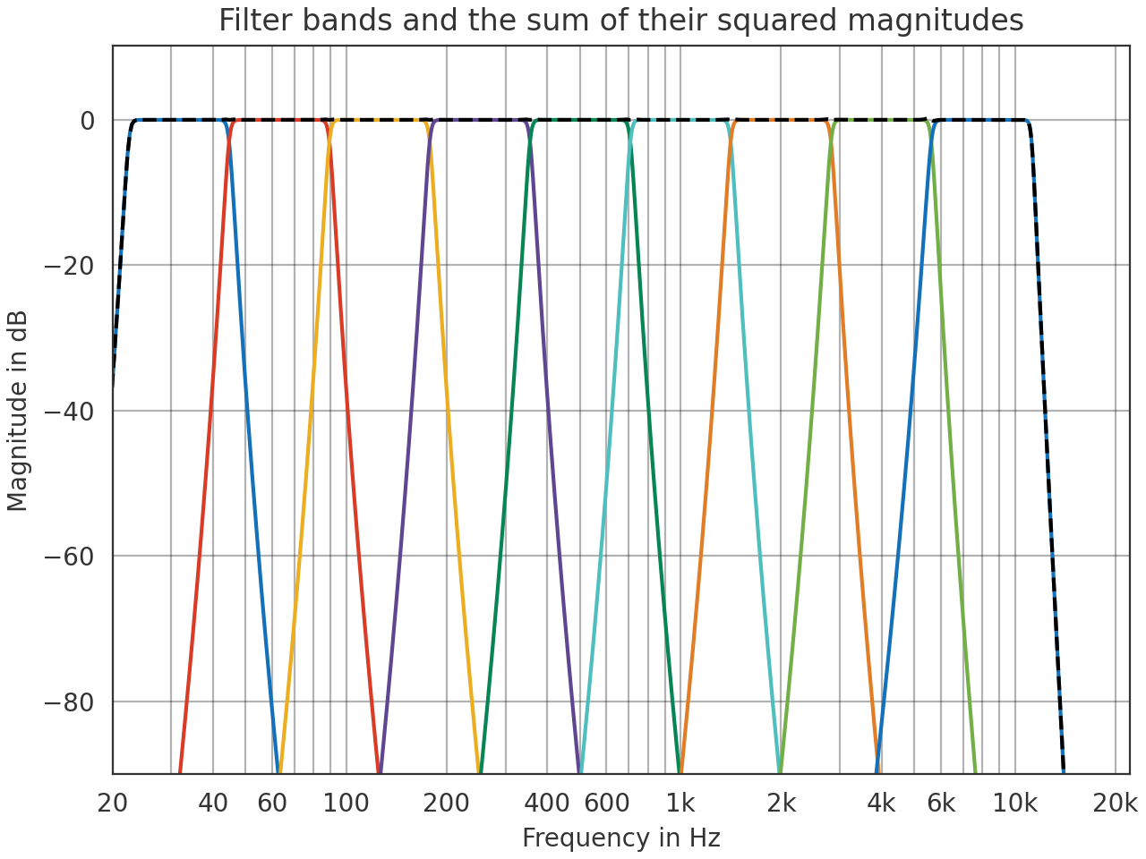
Filter an impulse into octave bands. The summed energy of all bands equals the energy of the input signal.
>>> import pyfar as pf
>>> import numpy as np
>>> import matplotlib.pyplot as plt
>>> # generate the data
>>> x = pf.signals.impulse(2**17)
>>> y = pf.dsp.filter.fractional_octave_bands(
...     x, 1, frequency_range=(20, 8e3))
>>> # frequency domain plot
>>> y_sum = pf.FrequencyData(
...     np.sum(np.abs(y.freq)**2, 0), y.frequencies)
>>> pf.plot.freq(y)
>>> ax = pf.plot.freq(y_sum, color='k', log_prefix=10, linestyle='--')
>>> ax.set_title(
...     "Filter bands and the sum of their squared magnitudes")
(
Source code,png,hires.png,pdf)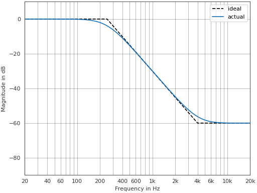
Show that the filters meet class 1 tolerance according to IEC 61260-1
>>> import pyfar as pf
>>> import numpy as np
>>> import matplotlib.pyplot as plt
>>>
>>> # get octave filter
>>> center_frequency = 1000
>>> num_fractions = 1
>>> octave_filter = pf.dsp.filter.fractional_octave_bands(
...     None, num_fractions, 44100,
...     (center_frequency, center_frequency))
>>>
>>> assert pf.dsp.filter.check_fractional_octave_band_filter_tolerance(
...     octave_filter, num_fractions,
...     (center_frequency, center_frequency), tolerance_class=1)
>>>
>>> # Class 1 tolerance after DIN EN 61260-1:2014, Table 1.
>>> lower, upper, frequencies = pf.constants.fractional_octave_filter_tolerance(
...         center_frequency, num_fractions, tolerance_class=1)
>>>
>>> # plot filter and tolerance
>>> ax = pf.plot.freq(octave_filter.impulse_response(2**14),
...                   color='k', label='Octave filter')
>>> ax.fill_between(
...     frequencies, lower, upper, facecolor=pf.plot.color('g'),
>>>     alpha=.25, label='Class 1 Tolerance region')
>>>
>>> ax.set_ylim(-40, 5)
>>> ax.set_xlim(.5*center_frequency, 2*center_frequency)
>>> ax.legend()
(
Source code,png,hires.png,pdf)
- pyfar.dsp.filter.fractional_octave_frequencies(num_fractions=1, frequency_range=(20, 20000.0), return_cutoff=False)[source]#
Return the octave center frequencies according to the IEC 61260:1:2014 standard.
For numbers of fractions other than
1and3, only the exact center frequencies are returned, since nominal frequencies are not specified by corresponding standards.- Parameters:
num_fractions (int, optional) – The number of bands an octave is divided into. Eg.,
1refers to octave bands and3to third octave bands. The default is1.frequency_range (array, tuple) – The lower and upper frequency limits, the default is
frequency_range=(20, 20e3).return_cutoff (bool, optional) – If
True, the lower and upper critical frequencies of the bandpass filters for each band are returned. The default isFalse.
- Returns:
nominal (array, float) – The nominal center frequencies are only defined for octave bands and third octave bands in the range between 25 Hz and 20 kHz. For all other cases,
Noneis returned.exact (array, float) – The exact center frequencies in Hz, resulting in a uniform distribution of frequency bands over the frequency range.
cutoff_freq (tuple, array, float) – The lower and upper critical frequencies in Hz of the bandpass filters for each band as a tuple corresponding to
(f_lower, f_upper).
- pyfar.dsp.filter.frequency_weighting_filter(signal, target_weighting: Literal['A', 'C'] = 'A', n_bins=100, error_weighting: Callable[[ndarray], ndarray] | None = None, sampling_rate: float | None = None, **kwargs)[source]#
Create and apply an A or C weighting filter.
The created SOS filter approximates the A or C weighting defined in IEC 61672-1 [13].
Note
This function will run a least-squares algorithm to iteratively approach the filter coefficients for the target weighting curve. The coefficients are cached, but only when the error_weighting and kwargs arguments are unused, which are unhashable. When using these parameters, it is faster to create the filter once and reuse it than calling this function repeatedly.
Note
When using default parameters for n_bins and error_weighting and no kwargs, the returned filter is compliant with a class 1 sound level meter as described in the standard for the sampling rates 48 kHz, 44.1 kHz, 16 kHz as well as these sampling rates multiplied by 2, 1/2, 4, 1/4, 8, and 1/8 each. For other arguments or sampling rates, the returned filter may not comply with class 1 requirements, in which case a warning will be printed.
- Parameters:
signal (Signal, None) – The signal to be filtered. Pass
Noneto create the filter without applying it.target_weighting (str, optional) – Specifies which frequency weighting curve to approximate. Must be either
"A"or"C". The default is"A".n_bins (int, optional) – At how many frequencies to evaluate the filter coefficients during optimization. Less frequencies means faster iterations, but potentially worse results. The evaluation frequencies are logarithmically spaced between 10 Hz and the Nyquist frequency. The default is
100.error_weighting (callable) – A function that can be used to emphasize the approximation errors in specific frequency ranges. The function should take a float array as argument, specifying the normalized frequencies between 0 and 1 (where 1 is the Nyquist frequency) to weight, and returns a float array as output containing the weights. By default the errors of all (logarithmically spaced) frequencies are equally weighted. This usually leads to larger errors for higher frequencies. By passing a function that emphasizes high frequencies, it is possible to reduce this effect and get a filter potentially closer to the target curve (see examples below). The default is
None.sampling_rate (float, conditionally optional) – The sampling rate of the returned filter. The default is
None.**kwargs (dict) – Keyword args that are passed to the
scipy.optimize.least_squarescall.
- Returns:
signal (Signal) – The filtered signal. Only returned if
sampling_rate = None.filter (FilterSOS) – The frequency weighting filter as SOS Filter object. Only returned if
signal = None. If weighting is'A'the filter order will be 6.'C'weighting will return a filter of order 4.
References
Examples
Create and apply an A weighting filter to white noise.
>>> import pyfar as pf
>>> import matplotlib.pyplot as plt
>>> noise = pf.dsp.normalize(pf.signals.noise(10000), domain="freq")
>>> weighting_filter = pf.dsp.filter.frequency_weighting_filter(
...     None, "A", sampling_rate=noise.sampling_rate)
>>> weighted_noise = weighting_filter.process(noise)
>>> pf.plot.freq(noise, label="unweighted noise")
>>> pf.plot.freq(
...     weighting_filter.impulse_response(10000),
...     label="weighting filter")
>>> pf.plot.freq(weighted_noise, label="A weighted noise")
>>> plt.ylim(-45, 5)
>>> plt.legend()
(
Source code,png,hires.png,pdf)
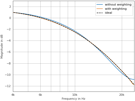
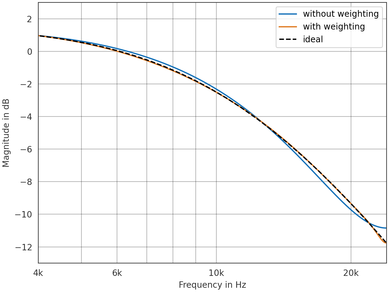
Use the
error_weightingparameter to emphasize filter accuracy near the Nyquist frequency. Note that the results depend on the sampling rate and your device (operating system, hardware).>>> import pyfar as pf >>> import matplotlib.pyplot as plt >>> import numpy as np >>> impulse = pf.signals.impulse(1000, sampling_rate=48000) >>> no_weighting = pf.dsp.filter.frequency_weighting_filter(impulse) >>> with_weighting = pf.dsp.filter.frequency_weighting_filter( ... impulse, error_weighting=lambda nf: 100**nf) >>> pf.plot.freq(no_weighting, c="b", label="without weighting") >>> pf.plot.freq(with_weighting, c="o", label="with weighting") >>> f = np.logspace(1, 4.4, 100) >>> ideal = pf.constants.frequency_weighting_curve("A", f) >>> plt.plot(f, ideal, linestyle="--", c="black", label="ideal") >>> plt.legend() >>> plt.ylim(-13, 3) >>> plt.xlim(4e3, 24e3) >>> plt.show()
(
Source code,png,hires.png,pdf)
- pyfar.dsp.filter.high_shelf(signal, frequency, gain, order, shelf_type='I', sampling_rate=None)[source]#
Create and/or apply first or second order high shelf filter.
Uses the implementation of [14].
- Parameters:
signal (Signal, None) – The Signal to be filtered. Pass
Noneto create the filter without applying it.frequency (number) – Characteristic frequency of the shelf in Hz.
gain (number) – Gain of the shelf in dB.
order (number) – The shelf order. Must be
1or2.shelf_type (str) –
Defines the characteristic frequency. The default is
'I'.'I'Defines the characteristic frequency 3 dB below the gain value if the gain is positive and 3 dB above the gain value if the gain is negative.
'II'Defines the characteristic frequency at 3 dB if the gain is positive and at -3 dB if the gain is negative.
'III'Defines the characteristic frequency at gain/2 dB.
For types
IandIIthe absolute value of the gain must be sufficiently large (> 9 dB) to set the characteristic frequency according to the above rules with an error below 0.5 dB. For smaller absolute gain values the gain at the characteristic frequency becomes less accurate. For typeIIIthe characteristic frequency is always set correctly.sampling_rate (None, number) – The sampling rate in Hz. Only required if signal is
None. The default isNone.
- Returns:
signal (Signal) – The filtered signal. Only returned if
sampling_rate = None.filter (FilterIIR) – Filter object. Only returned if
signal = None.
References
- pyfar.dsp.filter.high_shelf_cascade(signal, frequency, frequency_type='lower', gain=None, slope=None, bandwidth=None, N=None, sampling_rate=None)[source]#
Create and apply constant slope filter from cascaded 2nd order high shelves.
The filters - also known as High-Schultz filters (cf. [15]) - are defined by their characteristic frequency, gain, slope, and bandwidth. Two out of the three parameter gain, slope, and bandwidth must be specified, while the third parameter is calculated as
gain = bandwidth * slopebandwidth = abs(gain/slope)slope = gain/bandwidthNote
The bandwidth must be at least 1 octave to obtain a good approximation of the desired frequency response. Make sure to specify the parameters gain, slope, and bandwidth accordingly.
- Parameters:
signal (Signal, None) – The Signal to be filtered. Pass
Noneto create the filter without applying it.frequency (number) – Characteristic frequency in Hz (see frequency_type)
frequency_type (string) –
Defines how frequency is used
'upper'frequency gives the upper characteristic frequency. In this case the lower characteristic frequency is given by
2**bandwidth / frequency'lower'frequency gives the lower characteristic frequency. In this case the upper characteristic frequency is given by
2**bandwidth * frequency
gain (number) – The filter gain in dB. The default is
None, which calculates the gain from the slope and bandwidth (must be given if gain isNone).slope (number) – Filter slope in dB per octave, with positive values denoting a rising filter slope and negative values denoting a falling filter slope. The default is
None, which calculates the slope from the gain and bandwidth (must be given if slope isNone).bandwidth (number) – The bandwidth of the filter in octaves. The default is
None, which calculates the bandwidth from gain and slope (must be given if bandwidth isNone).N (int) – Number of shelf filters that are cascaded. The default is
None, which calculated the minimumNthat is required to satisfy Eq. (11) in Schultz et al. 2020, i.e., the minimumNthat is required for a good approximation of the ideal filter response.sampling_rate (None, number) – The sampling rate in Hz. Only required if signal is
None. The default isNone.
- Returns:
signal (
Signal,FilterSOS) – The filtered signal (returned ifsampling_rate = None) or the Filter object (returned ifsignal = None).N (int) – The number of shelf filters that were cascaded
ideal (
FrequencyData) – The ideal, piece-wise magnitude response of the filter
References
Examples
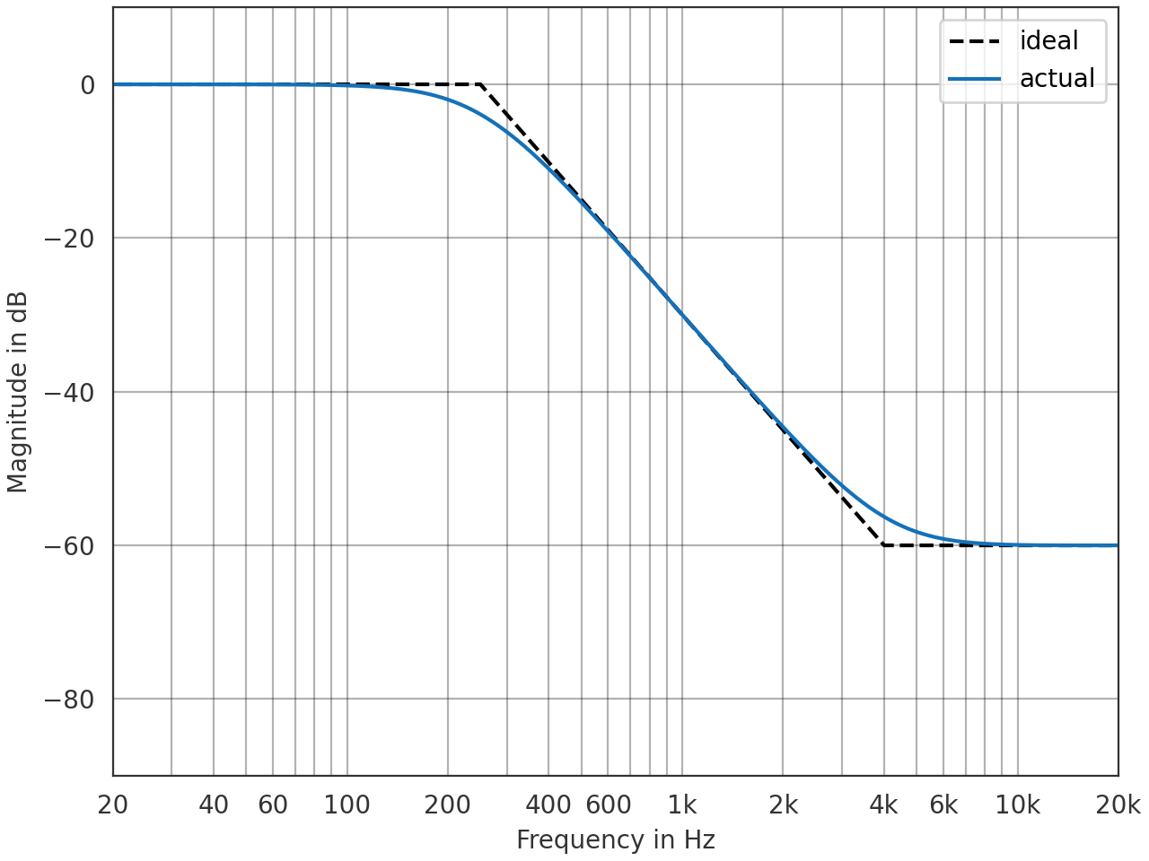
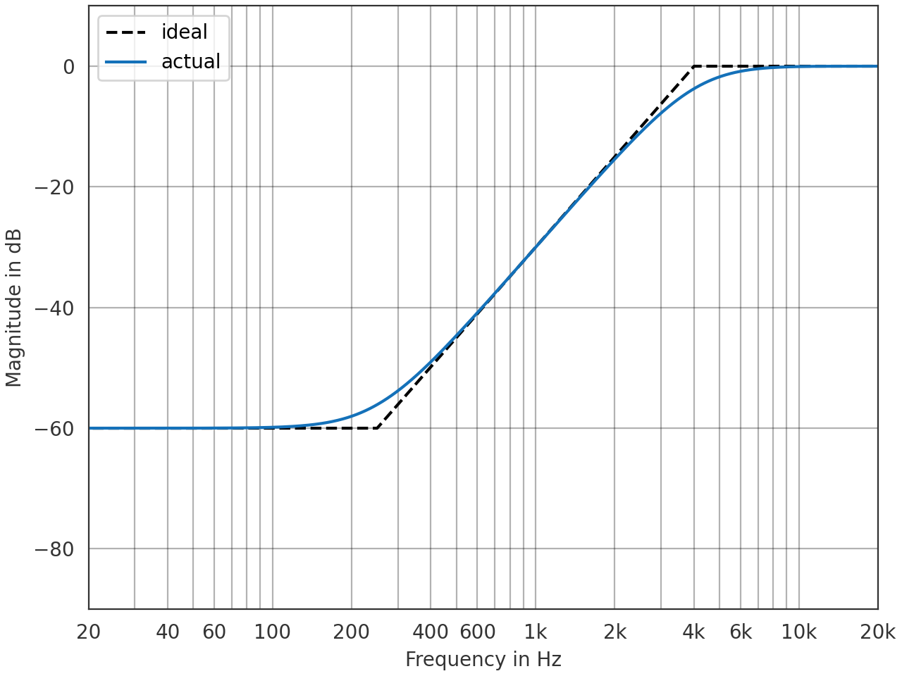
Generate a filter with a bandwith of 4 octaves and a gain of -60 dB and compare it to the piece-wise constant idealized magnitude response.
>>> import pyfar as pf
>>> import matplotlib.pyplot as plt
>>>
>>> impulse = pf.signals.impulse(40e3, sampling_rate=40000)
>>> impulse, N, ideal = pf.dsp.filter.high_shelf_cascade(
>>>     impulse, 250, "lower", -60, None, 4)
>>>
>>> pf.plot.freq(ideal, c='k', ls='--', label="ideal")
>>> pf.plot.freq(impulse, label="actual")
>>> plt.legend()
(
Source code,png,hires.png,pdf)
- pyfar.dsp.filter.high_shelve(signal, frequency, gain, order, shelve_type='I', sampling_rate=None)[source]#
high_shelvewill be deprecated in pyfar 0.9.0 in favor ofhigh_shelf. Create and/or apply first or second order high shelf filter.Uses the implementation of [16].
- Parameters:
signal (Signal, None) – The Signal to be filtered. Pass
Noneto create the filter without applying it.frequency (number) – Characteristic frequency of the shelf in Hz.
gain (number) – Gain of the shelf in dB.
order (number) – The shelf order. Must be
1or2.shelve_type (str) –
Defines the characteristic frequency. The default is
'I'.'I'Defines the characteristic frequency 3 dB below the gain value if the gain is positive and 3 dB above the gain value if the gain is negative.
'II'Defines the characteristic frequency at 3 dB if the gain is positive and at -3 dB if the gain is negative.
'III'Defines the characteristic frequency at gain/2 dB.
For types
IandIIthe absolute value of the gain must be sufficiently large (> 9 dB) to set the characteristic frequency according to the above rules with an error below 0.5 dB. For smaller absolute gain values the gain at the characteristic frequency becomes less accurate. For typeIIIthe characteristic frequency is always set correctly.sampling_rate (None, number) – The sampling rate in Hz. Only required if signal is
None. The default isNone.
- Returns:
signal (Signal) – The filtered signal. Only returned if
sampling_rate = None.filter (FilterIIR) – Filter object. Only returned if
signal = None.
References
- pyfar.dsp.filter.high_shelve_cascade(signal, frequency, frequency_type='lower', gain=None, slope=None, bandwidth=None, N=None, sampling_rate=None)[source]#
high_shelve_cascadewill be deprecated in pyfar 0.9.0 in favor ofhigh_shelf_cascade. Create and apply constant slope filter from cascaded 2nd order high shelves.The filters - also known as High-Schultz filters (cf. [17]) - are defined by their characteristic frequency, gain, slope, and bandwidth. Two out of the three parameter gain, slope, and bandwidth must be specified, while the third parameter is calculated as
gain = bandwidth * slopebandwidth = abs(gain/slope)slope = gain/bandwidth- Parameters:
signal (Signal, None) – The Signal to be filtered. Pass
Noneto create the filter without applying it.frequency (number) – Characteristic frequency in Hz (see frequency_type)
frequency_type (string) –
Defines how frequency is used
'upper'frequency gives the upper characteristic frequency. In this case the lower characteristic frequency is given by
2**bandwidth / frequency'lower'frequency gives the lower characteristic frequency. In this case the upper characteristic frequency is given by
2**bandwidth * frequency
gain (number) – The filter gain in dB. The default is
None, which calculates the gain from the slope and bandwidth (must be given if gain isNone).slope (number) – Filter slope in dB per octave, with positive values denoting a rising filter slope and negative values denoting a falling filter slope. The default is
None, which calculates the slope from the gain and bandwidth (must be given if slope isNone).bandwidth (number) – The bandwidth of the filter in octaves. The default is
None, which calculates the bandwidth from gain and slope (must be given if bandwidth isNone).N (int) – Number of shelf filters that are cascaded. The default is
None, which calculated the minimumNthat is required to satisfy Eq. (11) in Schultz et al. 2020, i.e., the minimumNthat is required for a good approximation of the ideal filter response.sampling_rate (None, number) – The sampling rate in Hz. Only required if signal is
None. The default isNone.
- Returns:
signal (
Signal,FilterSOS) – The filtered signal (returned ifsampling_rate = None) or the Filter object (returned ifsignal = None).N (int) – The number of shelf filters that were cascaded
ideal (
FrequencyData) – The ideal, piece-wise magnitude response of the filter
References
Examples
Generate a filter with a bandwith of 4 octaves and a gain of -60 dB and compare it to the piece-wise constant idealized magnitude response.
>>> import pyfar as pf
>>> import matplotlib.pyplot as plt
>>>
>>> impulse = pf.signals.impulse(40e3, sampling_rate=40000)
>>> impulse, N, ideal = pf.dsp.filter.high_shelf_cascade(
>>>     impulse, 250, "lower", -60, None, 4)
>>>
>>> pf.plot.freq(ideal, c='k', ls='--', label="ideal")
>>> pf.plot.freq(impulse, label="actual")
>>> plt.legend()
(
Source code,png,hires.png,pdf)
- pyfar.dsp.filter.low_shelf(signal, frequency, gain, order, shelf_type='I', sampling_rate=None)[source]#
Create and apply first or second order low shelf filter.
Uses the implementation of [18].
- Parameters:
signal (Signal, None) – The Signal to be filtered. Pass
Noneto create the filter without applying it.frequency (number) – Characteristic frequency of the shelf in Hz.
gain (number) – Gain of the shelf in dB.
order (number) – The shelf order. Must be
1or2.shelf_type (str) –
Defines the characteristic frequency. The default is
'I'.'I'Defines the characteristic frequency 3 dB below the gain value if the gain is positive and 3 dB above the gain value if the gain is negative.
'II'Defines the characteristic frequency at 3 dB if the gain is positive and at -3 dB if the gain is negative.
'III'Defines the characteristic frequency at gain/2 dB.
For types
IandIIthe absolute value of the gain must be sufficiently large (> 9 dB) to set the characteristic frequency according to the above rules with an error below 0.5 dB. For smaller absolute gain values the gain at the characteristic frequency becomes less accurate. For typeIIIthe characteristic frequency is always set correctly.sampling_rate (None, number) – The sampling rate in Hz. Only required if signal is
None. The default isNone.
- Returns:
signal (Signal) – The filtered signal. Only returned if
sampling_rate = None.filter (FilterIIR) – Filter object. Only returned if
signal = None.
References
- pyfar.dsp.filter.low_shelf_cascade(signal, frequency, frequency_type='upper', gain=None, slope=None, bandwidth=None, N=None, sampling_rate=None)[source]#
Create and apply constant slope filter from cascaded 2nd order low shelves.
The filters - also known as Low-Schultz filters (cf. [19]) - are defined by their characteristic frequency, gain, slope, and bandwidth. Two out of the three parameter gain, slope, and bandwidth must be specified, while the third parameter is calculated as
gain = -bandwidth * slopebandwidth = abs(gain/slope)slope = -gain/bandwidthNote
The bandwidth must be at least 1 octave to obtain a good approximation of the desired frequency response. Make sure to specify the parameters gain, slope, and bandwidth accordingly.
- Parameters:
signal (Signal, None) – The Signal to be filtered. Pass
Noneto create the filter without applying it.frequency (number) – Characteristic frequency in Hz (see frequency_type)
frequency_type (string) –
Defines how frequency is used
'upper'frequency gives the upper characteristic frequency. In this case the lower characteristic frequency is given by
2**bandwidth / frequency'lower'frequency gives the lower characteristic frequency. In this case the upper characteristic frequency is given by
2**bandwidth * frequency
gain (number) – The filter gain in dB. The default is
None, which calculates the gain from the slope and bandwidth (must be given if gain isNone).slope (number) – Filter slope in dB per octave, with positive values denoting a rising filter slope and negative values denoting a falling filter slope. The default is
None, which calculates the slope from the gain and bandwidth (must be given if slope isNone).bandwidth (number) – The bandwidth of the filter in octaves. The default is
None, which calculates the bandwidth from gain and slope (must be given if bandwidth isNone).N (int) – Number of shelf filters that are cascaded. The default is
None, which calculated the minimumNthat is required to satisfy Eq. (11) in Schultz et al. 2020, i.e., the minimumNthat is required for a good approximation of the ideal filter response.sampling_rate (None, number) – The sampling rate in Hz. Only required if signal is
None. The default isNone.
- Returns:
signal (
Signal,FilterSOS) – The filtered signal (returned ifsampling_rate = None) or the Filter object (returned ifsignal = None).N (int) – The number of shelf filters that were cascaded
ideal (
FrequencyData) – The ideal, piece-wise magnitude response of the filter
References
Examples
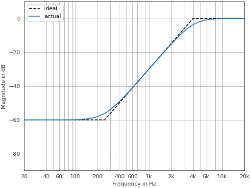
Generate a filter with a bandwith of 4 octaves and a gain of -60 dB and compare it to the piece-wise constant idealized magnitude response.
>>> import pyfar as pf
>>> import matplotlib.pyplot as plt
>>>
>>> impulse = pf.signals.impulse(40e3, sampling_rate=40000)
>>> impulse, N, ideal = pf.dsp.filter.low_shelf_cascade(
>>>     impulse, 4000, "upper", -60, None, 4)
>>>
>>> pf.plot.freq(ideal, c='k', ls='--', label="ideal")
>>> pf.plot.freq(impulse, label="actual")
>>> plt.legend()
(
Source code,png,hires.png,pdf)
- pyfar.dsp.filter.low_shelve(signal, frequency, gain, order, shelve_type='I', sampling_rate=None)[source]#
low_shelvewill be deprecated in pyfar 0.9.0 in favor oflow_shelf. Create and apply first or second order low shelf filter.Uses the implementation of [20].
- Parameters:
signal (Signal, None) – The Signal to be filtered. Pass
Noneto create the filter without applying it.frequency (number) – Characteristic frequency of the shelf in Hz.
gain (number) – Gain of the shelf in dB.
order (number) – The shelf order. Must be
1or2.shelve_type (str) –
Defines the characteristic frequency. The default is
'I'.'I'Defines the characteristic frequency 3 dB below the gain value if the gain is positive and 3 dB above the gain value if the gain is negative.
'II'Defines the characteristic frequency at 3 dB if the gain is positive and at -3 dB if the gain is negative.
'III'Defines the characteristic frequency at gain/2 dB.
For types
IandIIthe absolute value of the gain must be sufficiently large (> 9 dB) to set the characteristic frequency according to the above rules with an error below 0.5 dB. For smaller absolute gain values the gain at the characteristic frequency becomes less accurate. For typeIIIthe characteristic frequency is always set correctly.sampling_rate (None, number) – The sampling rate in Hz. Only required if signal is
None. The default isNone.
- Returns:
signal (Signal) – The filtered signal. Only returned if
sampling_rate = None.filter (FilterIIR) – Filter object. Only returned if
signal = None.
References
- pyfar.dsp.filter.low_shelve_cascade(signal, frequency, frequency_type='upper', gain=None, slope=None, bandwidth=None, N=None, sampling_rate=None)[source]#
low_shelve_cascadewill be deprecated in pyfar 0.9.0 in favor oflow_shelf_cascade. Create and apply constant slope filter from cascaded 2nd order low shelves.The filters - also known as Low-Schultz filters (cf. [21]) - are defined by their characteristic frequency, gain, slope, and bandwidth. Two out of the three parameter gain, slope, and bandwidth must be specified, while the third parameter is calculated as
gain = -bandwidth * slopebandwidth = abs(gain/slope)slope = -gain/bandwidth- Parameters:
signal (Signal, None) – The Signal to be filtered. Pass
Noneto create the filter without applying it.frequency (number) – Characteristic frequency in Hz (see frequency_type)
frequency_type (string) –
Defines how frequency is used
'upper'frequency gives the upper characteristic frequency. In this case the lower characteristic frequency is given by
2**bandwidth / frequency'lower'frequency gives the lower characteristic frequency. In this case the upper characteristic frequency is given by
2**bandwidth * frequency
gain (number) – The filter gain in dB. The default is
None, which calculates the gain from the slope and bandwidth (must be given if gain isNone).slope (number) – Filter slope in dB per octave, with positive values denoting a rising filter slope and negative values denoting a falling filter slope. The default is
None, which calculates the slope from the gain and bandwidth (must be given if slope isNone).bandwidth (number) – The bandwidth of the filter in octaves. The default is
None, which calculates the bandwidth from gain and slope (must be given if bandwidth isNone).N (int) – Number of shelf filters that are cascaded. The default is
None, which calculated the minimumNthat is required to satisfy Eq. (11) in Schultz et al. 2020, i.e., the minimumNthat is required for a good approximation of the ideal filter response.sampling_rate (None, number) – The sampling rate in Hz. Only required if signal is
None. The default isNone.
- Returns:
signal (
Signal,FilterSOS) – The filtered signal (returned ifsampling_rate = None) or the Filter object (returned ifsignal = None).N (int) – The number of shelf filters that were cascaded
ideal (
FrequencyData) – The ideal, piece-wise magnitude response of the filter
References
Examples
Generate a filter with a bandwith of 4 octaves and a gain of -60 dB and compare it to the piece-wise constant idealized magnitude response.
>>> import pyfar as pf
>>> import matplotlib.pyplot as plt
>>>
>>> impulse = pf.signals.impulse(40e3, sampling_rate=40000)
>>> impulse, N, ideal = pf.dsp.filter.low_shelf_cascade(
>>>     impulse, 4000, "upper", -60, None, 4)
>>>
>>> pf.plot.freq(ideal, c='k', ls='--', label="ideal")
>>> pf.plot.freq(impulse, label="actual")
>>> plt.legend()
(
Source code,png,hires.png,pdf)
- pyfar.dsp.filter.notch(signal, center_frequency, quality, sampling_rate=None)[source]#
Create and apply or return a second order IIR notch filter.
A notch filter is a band-stop filter with a narrow bandwidth (high quality factor). It rejects a narrow frequency band around the center frequency with a gain of 0 (\(-\infty\) dB) at the center frequency and leaves the rest of the spectrum little changed with gains close to 1 (0 dB) [22]. Wrapper for
scipy.signal.iirnotch.- Parameters:
signal (Signal, None) – The Signal to be filtered. Pass
Noneto create the filter without applying it.center_frequency (number) – Frequency in Hz at which the magnitude response will be 0 (\(-\infty\) dB).
quality (number) – The quality characterizes notch filter -3 dB bandwidth relative to its center frequency (both in Hz), i.e,
quality = center_frequency/bandwidth.sampling_rate (None, number) – The sampling rate in Hz. Only required if signal is
None. The default isNone.
- Returns:
output – The function returns a filtered version of the input signal if
sampling_rate = Noneor the filter itself ifsignal = None.- Return type:
References
- pyfar.dsp.filter.reconstructing_fractional_octave_bands(signal, num_fractions=1, frequency_range=(63, 16000), overlap=1, slope=0, n_samples=4096, sampling_rate=None)[source]#
Create and/or apply an amplitude preserving fractional octave filter bank.
Note
This filter bank has -6 dB cut-off frequencies. For sufficient lengths of
'n_samples', the summed output of the filter bank equals the input signal, i.e., the filter bank is amplitude preserving (reconstructing). This is useful for analysis and synthesis applications such as room acoustical simulations. For an energy preserving filter bank with -3 dB cut-off frequencies seefractional_octave_bands.The filters have a linear phase with a delay of
n_samples/2and are windowed with a Hanning window to suppress side lobes of the finite filters. The magnitude response of the filters is designed similar to [23] with two exceptions:The magnitude response is designed using squared sine/cosine ramps to obtain -6 dB at the cut-off frequencies.
The overlap between the filters is calculated between the center and upper cut-off frequencies and not between the center and lower cut-off frequencies. This enables smaller pass-bands with unity gain, which might be advantageous for applications that apply analysis and resynthesis.
- Parameters:
signal (Signal, None) – The Signal to be filtered. Pass
Noneto create the filter without applying it.num_fractions (int, optional) – Octave fraction, e.g.,
3for third-octave bands. The default is1.frequency_range (tuple, optional) – Frequency range for fractional octave in Hz. The default is
(63, 16000)overlap (float) – Band overlap of the filter slopes between 0 and 1. Smaller values yield wider pass-bands and steeper filter slopes. The default is
1.slope (int, optional) – Non-negative integer that defines the width and steepness of the filter slopes. Larger values yield wider pass-bands and steeper filter slopes. The default is
0.n_samples (int, optional) – Length of the filter in samples. Longer filters yield more exact filters. The default is
2**12.sampling_rate (int) – Sampling frequency in Hz. The default is
None. Only required ifsignal=None.
- Returns:
signal (Signal) – The filtered signal. Only returned if
sampling_rate = None.filter (FilterFIR) – FIR Filter object. Only returned if
signal = None.frequencies (np.ndarray) – Center frequencies of the filters. Return variable will be removed in pyfar 0.9.0. To get the fractional octave center frequencies, use
fractional_octave_frequenciesinstead.
References
Examples
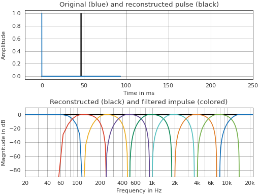
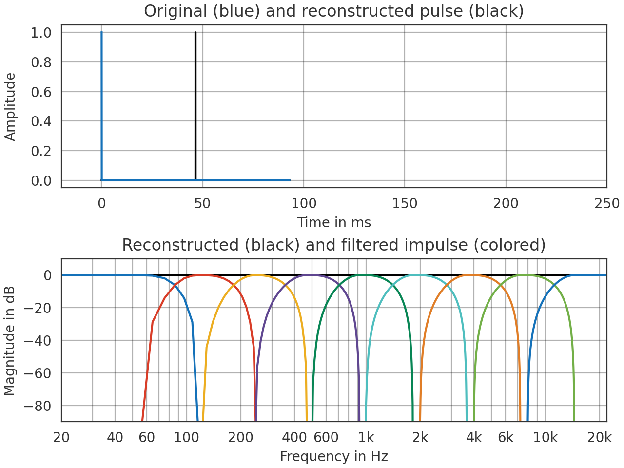
Filter and re-synthesize an impulse signal.
>>> import pyfar as pf
>>> import numpy as np
>>> import matplotlib.pyplot as plt
>>> # generate data
>>> x = pf.signals.impulse(2**12)
>>> y = pf.dsp.filter.reconstructing_fractional_octave_bands(x)[0]
>>> # get center frequencies
>>> f = pf.constants.fractional_octave_frequencies_exact(
...    frequency_range=(60, 16000))[0]
>>> y_sum = pf.Signal(np.sum(y.time, 0), y.sampling_rate)
>>> # time domain plot
>>> ax = pf.plot.time_freq(y_sum, color='k', unit='ms')
>>> pf.plot.time(x, ax=ax[0], unit='ms')
>>> ax[0].set_xlim(-20, 250)
>>> ax[0].set_title("Original (blue) and reconstructed pulse (black)")
>>> # frequency domain plot
>>> pf.plot.freq(y_sum, color='k', ax=ax[1])
>>> pf.plot.freq(y, ax=ax[1])
>>> ax[1].set_title(
...     "Reconstructed (black) and filtered impulse (colored)")
(
Source code,png,hires.png,pdf)