pyfar.dsp.fft¶

The discrete Fourier spectrum of an arbitrary, but band-limited signal $x(n)$ is defined as

$X(\mu) = \sum_{n=0}^{N-1} x(n) e^{-i 2 \pi \frac{\mu n}{N}}$

using a negative sign convention in the transform kernel $\kappa(\mu, n) = e^{-i 2 \pi \mu \frac{n}{N}}$ . Analogously, the discrete inverse Fourier transform is implemented as

$x(n) = \frac{1}{N} \sum_{\mu=0}^{N-1} X(\mu) e^{i2\pi\frac{\mu n}{N}}$

Pyfar uses a DFT implementation for purely real-valued time signals resulting in Fourier spectra with complex conjugate symmetry for negative and positive frequencies $X(\mu) = X(-\mu)^*$ . As a result, the left-hand side of the spectrum is discarded, yielding $X_R(\mu) = X(\mu) \mbox{ }\forall 0 \le \mu \le N/2$ . Complex valued time signals can be implemented, if required.

Normalization 1 ¶

pyfar implements five normalization that can be applied to spectra. The normalizations are available from normalization. Note that the time signals do not change regardless of the normalization.

Energy Signals¶

For energy signals with finite energy, such as impulse responses, no normalization is required, that is the spectrum of a energy signal is equivalent to the right-hand spectrum of a real-valued time signal defined above. The coresponding normalization is 'none'.

Power Signals¶

For power signals however, which possess a finite power but infinite energy, a normalization for the time interval in which the signal is sampled, is chosen. In order for Parseval’s theorem to remain valid, the single sided needs to be multiplied by a factor of 2, compensating for the discarded part of the spectrum (cf. 1, Eq. 8). The coresponding normalization is 'unitary'. Additional normalizations can be applied to further scale the spectrum, e.g., according to the RMS value.

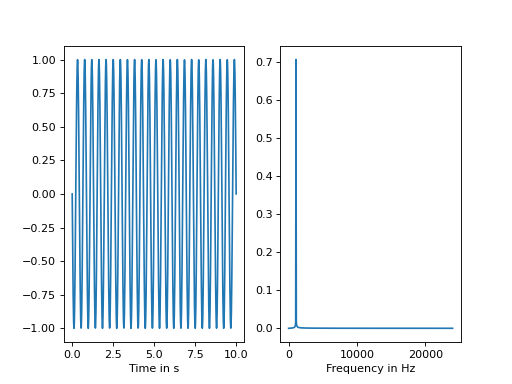
>>> import numpy as np
>>> from pyfar.dsp import fft
>>> import matplotlib.pyplot as plt
>>> # properties
>>> fft_normalization = "rms"
>>> n_samples = 1024
>>> sampling_rate = 48e3
>>> frequency = 100
>>> times = np.linspace(0, 10, n_samples)
>>> freqs = fft.rfftfreq(n_samples, 48e3)
>>> # generate data
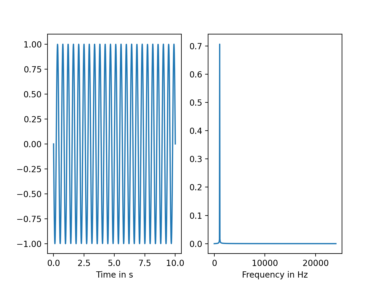
>>> sine = np.sin(times * 2*np.pi * frequency)
>>> spec = fft.rfft(sine, n_samples, sampling_rate, fft_normalization)
>>> # plot time and frequency data
>>> plt.subplot(1, 2, 1)
>>> plt.plot(times, sine)
>>> ax = plt.gca()
>>> ax.set_xlabel('Time in s')
>>> plt.subplot(1, 2, 2)
>>> plt.plot(freqs, np.abs(spec))
>>> ax = plt.gca()
>>> ax.set_xlabel('Frequency in Hz')
>>> plt.show()

(Source code, png, hires.png, pdf)

References

1(1,2,3,4,5,6,7,8,9,10): J. Ahrens, C. Andersson, P. Höstmad, and W. Kropp, “Tutorial on Scaling of the Discrete Fourier Transform and the Implied Physical Units of the Spectra of Time-Discrete Signals,” Vienna, Austria, May 2020, p. e-Brief 600.

Functions:

`irfft`(spec, n_samples, sampling_rate, fft_norm)	Calculate the IFFT of a axis-symmetric Fourier spectum.
`normalization`(spec, n_samples, sampling_rate)	Normalize spectrum.
`rfft`(data, n_samples, sampling_rate, fft_norm)	Calculate the FFT of a real-valued time-signal.
`rfftfreq`(n_samples, sampling_rate)	Returns the positive discrete frequencies in the range $[0, \text{sampling\_rate}/2]$ for which the FFT of a real valued time-signal with n_samples is calculated.

pyfar.dsp.fft.irfft(spec, n_samples, sampling_rate, fft_norm)[source]¶

Calculate the IFFT of a axis-symmetric Fourier spectum. The function takes only the right-hand side of the spectrum and returns a real-valued time signal. The normalization distinguishes between energy and power signals. Energy signals are not normalized by their number of samples. Power signals are normalized by their effective value as well as compensated for the missing energy from the left-hand side of the spectrum. This ensures that the energy of the time signal and the right-hand side of the spectrum are equal and thus fulfill Parseval’s theorem.

Parameters

spec (array, complex) – The complex valued right-hand side of the spectrum with dimensions (…, n_bins)
n_samples (int) – The number of samples in the corresponding tim signal. This is crucial to allow for the correct transform of time signals with an odd number of samples.
sampling_rate (number) – sampling rate in Hz
fft_norm ('unitary', 'amplitude', 'rms', 'power', 'psd') – See documentaion of normalization.

Returns

data – Array containing the time domain signal with dimensions (…, n_samples)

Return type

array, double

pyfar.dsp.fft.normalization(spec, n_samples, sampling_rate, fft_norm='none', inverse=False, single_sided=True, window=None)[source]¶

Normalize spectrum.

Apply normalizations defined in 1 to the DFT spectrum. Note that, the phase is maintained in all cases, i.e., instead of taking the squared absolute values in Eq. (5-6), the complex spectra are multiplied with their absolute values.

Parameters

spec (numpy array) – N dimensional array which has the frequency bins in the last dimension. E.g., spec.shape == (10,2,129) holds 10 times 2 spectra with 129 frequency bins each.
n_samples (int) – number of samples of the corresponding time signal
sampling_rate (number) – sampling rate of the corresponding time signal in Hz
fft_norm (string, optional) –

‘none’
Do not apply any normalization

’unitary’
Multiplied single sided spectra by factor two as in 1 Eq. (8) (except for 0 Hz and the Nyquist frequency at half the sampling rate)

’amplitude’
scale spec by 1/n_samples as in 1 Eq. (4)

’rms’
scale spec by $1/\sqrt{2}$ as in 1 Eq. (10)

’power’
scale the power spectrum by 1/n_samples**2 as in 1 Eq. (5)

’psd’
scale the power spectrum by 1/(sampling_rate * n_samples as in 1 Eq. (6)

Note that the unitary normalization is also applied for amplitude, rms, power, and psd if the input spectrum is single sided (See below).
inverse (bool, optional) – apply the inverse normalization. The default is False.
single_sided (bool, optional) – denotes if spec is a single sided spectrum up to half the sampling rate or a both sided (full) spectrum. If single_sided=True the normalization according to 1 Eq. (8) is unless fft_norm='none'. The default is True.
window (None, array like) – window that was applied to the time signal before performing the FFT. window must be an array like with n_samples and affects the normalization as in 1 Eqs. (11-13). The default is None, which denotes that no window was applied.

Returns

spec – normalized input spectrum

Return type

numpy array

pyfar.dsp.fft.rfft(data, n_samples, sampling_rate, fft_norm)[source]¶

Calculate the FFT of a real-valued time-signal. The function returns only the right-hand side of the axis-symmetric spectrum. The normalization distinguishes between energy and power signals. Energy signals are not normalized in the forward transform. Power signals are normalized by their number of samples and to their effective value as well as compensated for the missing energy from the left-hand side of the spectrum. This ensures that the energy of the time signal and the right-hand side of the spectrum are equal and thus fulfill Parseval’s theorem.

Parameters

data (array, double) – Array containing the time domain signal with dimensions (…, n_samples)
n_samples (int) – The number of samples
sampling_rate (number) – sampling rate in Hz
fft_norm ('unitary', 'amplitude', 'rms', 'power', 'psd') – See documentation of normalization.

Returns

spec – The complex valued right-hand side of the spectrum with dimensions (…, n_bins)

Return type

array, complex

pyfar.dsp.fft.rfftfreq(n_samples, sampling_rate)[source]¶

Returns the positive discrete frequencies in the range $[0, \text{sampling\_rate}/2]$ for which the FFT of a real valued time-signal with n_samples is calculated. If the number of samples $N$ is even the number of frequency bins will be $2/N+1$ , if $N$ is odd, the number of bins will be $(N+1)/2$ .

Parameters

n_samples (int) – The number of samples in the signal
sampling_rate (int) – The sampling rate of the signal

Returns

frequencies – The positive discrete frequencies in Hz for which the FFT is calculated.

Return type

array, double

pyfar.dsp.fft¶

Normalization 1¶

Energy Signals¶

Power Signals¶

Normalization 1 ¶