
pyfar.dsp#
Digital signal processing functions.
Classes:
|
Interpolate an incomplete spectrum to a complete single sided spectrum. |
Class for frequency-dependent regularized inversion. |
Functions:
|
Average multi-channel signals. |
|
Convolve two signals. |
|
Compute the channel-wise correlation function between signals. |
|
Convert data of the selected signal domain into decibels (dB). |
|
Calculate transfer functions by spectral deconvolution of two signals. |
|
Computes the channel wise energy in the time domain. |
|
Find the delay in sub-sample values of an impulse response. |
|
Find the start sample of an impulse response. |
|
Apply fractional time shift to input data. |
|
Returns the group delay of a signal in samples. |
Return a shape parameter beta to create kaiser window based on desired side lobe suppression in dB. |
|
|
Set the phase to a linear phase with a specified group delay. |
|
Calculate the minimum phase equivalent of a finite impulse response. |
|
Apply a normalization. |
|
Pad a signal with zeros in the time domain. |
|
Returns the phase for a given signal object. |
|
Compute the power of a signal. |
|
Invert the spectrum of a signal applying frequency dependent regularization. |
|
Resample signal to new sampling rate. |
|
Compute the root mean square (RMS) of a signal. |
|
Smooth spectrum with a fractional octave width. |
|
Soft limiting the magniude spectrum. |
|
Compute the magnitude spectrum versus time. |
|
|
|
Apply a cyclic or linear time-shift to a signal. |
|
Apply time window to signal. |
|
Wraps phase to 2 pi. |
|
Calculate zero phase signal. |
- class pyfar.dsp.InterpolateSpectrum(data, method, kind, fscale='linear', clip=False)[source]#
Bases:
objectInterpolate an incomplete spectrum to a complete single sided spectrum.
This is intended to interpolate transfer functions, for example sparse spectra that are defined only at octave frequencies or incomplete spectra from numerical simulations.
- Parameters:
data (FrequencyData) – Input data to be interpolated.
method (string) –
Specifies the input data for the interpolation
'complex'Separate interpolation of the real and imaginary part
'magnitude_phase'Separate interpolation if the magnitude and unwrapped phase values
'magnitude'Interpolate the magnitude values only. Results in a zero phase signal, which is symmetric around the first sample. This phase response might not be ideal for many applications. Minimum and linear phase responses can be generated with
minimum_phaseandlinear_phase.
kind (tuple) –
Three element tuple
('first', 'second', 'third')that specifies the kind of inter/extrapolation below the lowest frequency (first), between the lowest and highest frequency (second), and above the highest frequency (third).The individual strings have to be
'zero',slinear,'quadratic','cubic'Spline interpolation of zeroth, first, second or third order
'previous','next'Simply return the previous or next value of the point
'nearest-up','nearest'Differ when interpolating half-integers (e.g. 0.5, 1.5) in that
'nearest-up'rounds up and'nearest'rounds down.
The interpolation is done using
scipy.interpolate.interp1d.fscale (string, optional) –
'linear'Interpolate on a linear frequency axis.
'log'Interpolate on a logarithmic frequency axis.
The default is
'linear'.clip (bool, tuple) – The interpolated magnitude response is clipped to the range specified by this two element tuple. E.g.,
clip=(0, 1)will assure that no values smaller than 0 and larger than 1 occur in the interpolated magnitude response. The clipping is applied after the interpolation. The default isFalsewhich does not clip the data.
- Returns:
interpolator – The interpolator can be called to interpolate the data (see examples below). It returns a
Signaland has the following parameters- n_samplesint
Length of the interpolated time signal in samples
- sampling_rate: int
Sampling rate of the output signal in Hz
- showbool, optional
Show a plot of the input and output data. The default is
False.
- Return type:
Examples
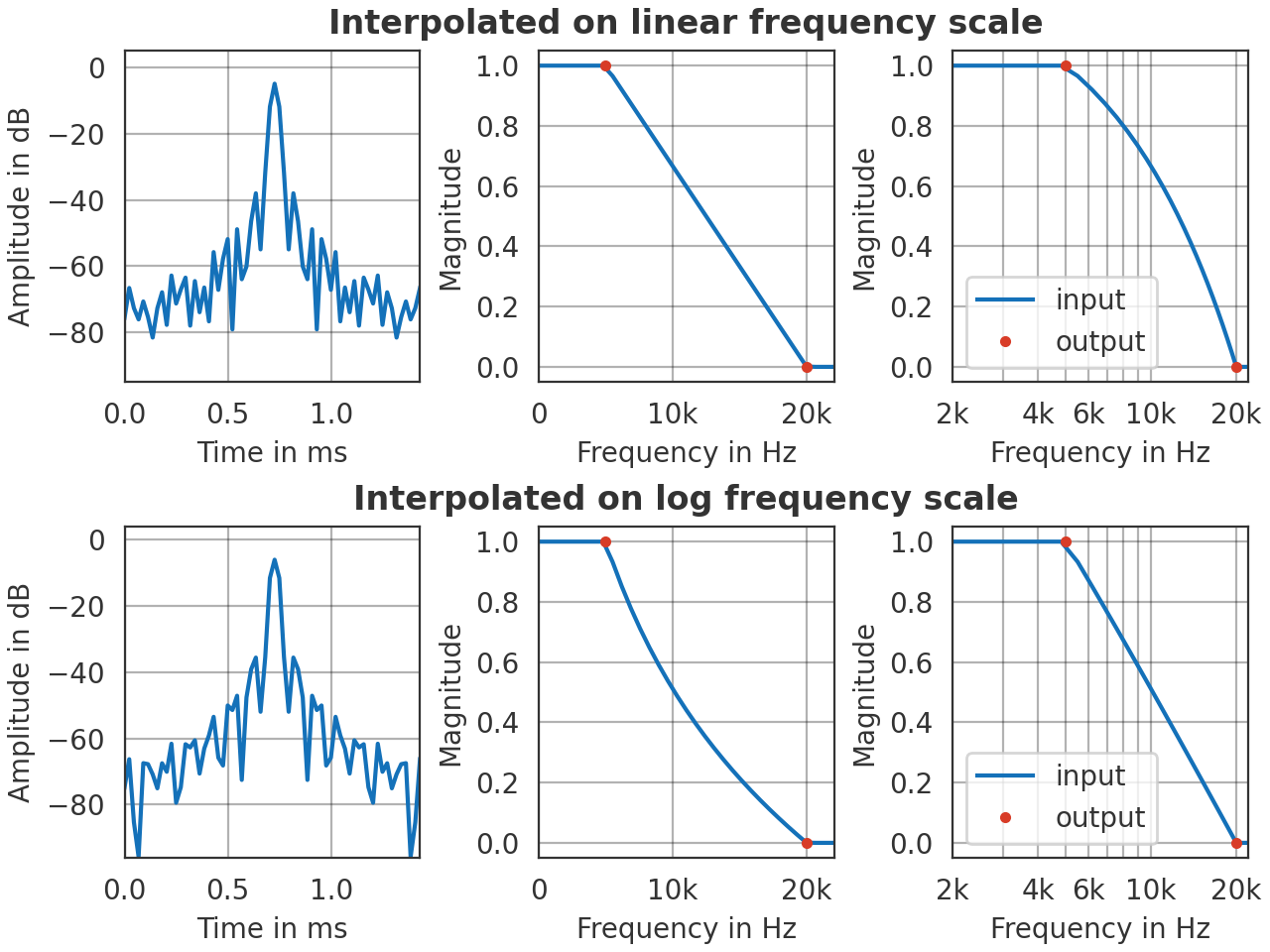
Interpolate a magnitude spectrum, add an artificial linear phase and inspect the results. Note that a similar plot can be created by the interpolator object by
signal = interpolator(64, 44100, show=True)>>> import pyfar as pf >>> import matplotlib.pyplot as plt >>> import numpy as np >>> >>> pf.plot.use() >>> _, ax = plt.subplots(2, 3) >>> >>> # generate data >>> data = pf.FrequencyData([1, 0], [5e3, 20e3]) >>> >>> # interpolate and plot >>> for ff, fscale in enumerate(["linear", "log"]): >>> interpolator = pf.dsp.InterpolateSpectrum( ... data, 'magnitude', ('nearest', 'linear', 'nearest'), ... fscale) >>> >>> # interpolate to 64 samples linear phase impulse response >>> signal = interpolator(64, 44100) >>> signal = pf.dsp.linear_phase(signal, 32) >>> >>> # time signal (linear and logarithmic amplitude) >>> pf.plot.time(signal, ax=ax[ff, 0], unit='ms', dB=True) >>> # frequency plot (linear x-axis) >>> pf.plot.freq( ... signal, dB=False, freq_scale="linear", ax=ax[ff, 1]) >>> pf.plot.freq(data, dB=False, freq_scale="linear", ... ax=ax[ff, 1], c='r', ls='', marker='.') >>> ax[ff, 1].set_xlim(0, signal.sampling_rate/2) >>> ax[ff, 1].set_title( ... f"Interpolated on {fscale} frequency scale") >>> # frequency plot (log x-axis) >>> pf.plot.freq(signal, dB=False, ax=ax[ff, 2], label='input') >>> pf.plot.freq(data, dB=False, ax=ax[ff, 2], ... c='r', ls='', marker='.', label='output') >>> ax[ff, 2].set_xlim(2e3, signal.sampling_rate/2) >>> ax[ff, 2].legend(loc='best')
(
Source code,png,hires.png,pdf)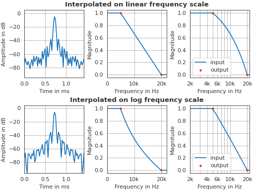
- class pyfar.dsp.RegularizedSpectrumInversion[source]#
Bases:
objectClass for frequency-dependent regularized inversion.
Regularized inversion limits the gain applied by an inverse filter. This can be useful to avoid extreme amplification when inverting a signal of limited bandwidth or containing notches in the spectrum.
The inverse is computed as [1]:
(1)#\[S^{-1}(f) = \frac{S^*(f)}{S^*(f)S(f) + \beta |\epsilon(f)|^2} D(f)\]with \(f\) being the frequency, \(S(f)\) the spectrum of the signal to be inverted, \(^*\) the complex conjugate, \(\epsilon(f)\) the regularization, and \(\beta\) a scalar to control the amount of regularization. \(D(f)\) denotes an optional target function.
The compensated system \(C = S(f)S^{-1}(f)\) approaches the target function in magnitude and phase. In many applications, the target function should contain a delay to make sure that \(S^{-1}(f)\) is causal. The larger \(\beta\) and \(\epsilon(f)\) are, the larger the deviation of \(C(f)\) from the target \(D(f)\).
The inversion is done in two steps:
Define \(S(f)\), \(\epsilon(f)\), \(\beta\), and \(D(f)\) using one of the
from_...()methods listed below.Compute the inverse \(S(f)^{-1}\) using
invert
The parameters that are defined in the first step are often iteratively adjusted. Examples are given in the documentation of the
from_...()methods.References
Attributes:
Scaling \(\beta\) of regularization function \(\epsilon(f)\).
Numeric \(\beta\) value.
Invert signal using frequency-dependent regularized inversion.
Regularization \(\epsilon(f)\) without scaling by \(\beta\).
Signal \(S(f)\) to be inverted.
Target function \(D(f)\).
Methods:
from_frequency_range(signal, frequency_range)Regularization from a given frequency range.
from_magnitude_spectrum(signal, regularization)Regularization from a given magnitude spectrum.
- property beta#
Scaling \(\beta\) of regularization function \(\epsilon(f)\).
This can be
'energy','max','mean', or a number.To return the numeric \(\beta\) value used in the inversion as in equation (1), use the property
beta_value.
- property beta_value#
Numeric \(\beta\) value.
- classmethod from_frequency_range(signal, frequency_range, regularization_within=0, beta=1, target=None)[source]#
Regularization from a given frequency range.
Defines a frequency range within which the regularization \(\epsilon(f)\) is set to regularization_within. Outside the frequency range the regularization is \(\epsilon(f)=1\) and can be controlled using the beta parameter. The regularization factors are cross-faded using a raised cosine window function with a width of \(\sqrt{2}f\) above and below the given frequency range.
- Parameters:
signal (Signal) – Signal to be inverted.
frequency_range (array like) – Array like containing the lower and upper frequency limit in Hz.
regularization_within (float, optional) – Set regularization inside frequency range. The default is 0.
beta (float, string, optional) –
Beta parameter to control the scaling of the regularization as in equation (1). Can be a
numerical valueUsually between
0and1, with0being no regularization applied.'energy'Normalize the regularization to match the signal’s energy.
\(\beta = \frac{\frac{1}{N}\sum_{k=0}^{N-1}|S[k]|^2}{\frac{1}{N}\sum_{k=0}^{N-1}|\epsilon[k]|^2}\)
'max'Normalize the regularization \(\epsilon(f)\) to the maximum magnitude of a given signal \(S(f)\).
\(\beta = \frac{\max(|S(f)|)}{\max(|\epsilon(f)|)}\)
'mean'Normalize the regularization \(\epsilon(f)\) to the mean magnitude of a given signal \(S(f).\)
\(\beta = \frac{\text{mean}(|S(f)|)}{\text{mean}(|\epsilon(f)|)}\)
The default is
1.target (Signal, optional) – Target function for the regularization. The default
Noneuses a zero-phase spectrum with an amplitude of 1 as target, equal to an impulse in the time domain.
Examples
Invert a sine sweep with limited bandwidth and apply maximum normalization to the regularization function.
>>> import pyfar as pf
>>> import matplotlib.pyplot as plt
...
>>> sweep = pf.signals.exponential_sweep_freq(
...     2**16, [50, 16e3], 1000, 10e3)
...
>>> # Inversion
>>> Inversion = pf.dsp.RegularizedSpectrumInversion.from_frequency_range(
>>>     sweep, [50, 16e3], beta='max')
>>> inverted = Inversion.invert
...
>>> # Obtain the scaled regularization function
>>> regularization = Inversion.regularization * Inversion.beta_value
...
>>> pf.plot.use()
>>> fig, axes = plt.subplots(2,1)
>>> pf.plot.freq(sweep, ax=axes[0], label='sweep')
>>> pf.plot.freq(regularization, ax=axes[0], label='regularization')
>>> axes[0].axvline(50, color='k', linestyle='--',
...     label='frequency range')
>>> axes[0].axvline(16e3, color='k', linestyle='--')
>>> axes[0].legend(loc='lower center')
...
>>> pf.plot.freq(inverted, ax=axes[1], color='p',
...     label='inverted with regulariztion')
>>> pf.plot.freq(1 / (sweep+1e-10), ax=axes[1], color='y',
...     linestyle=':', label='inverted without regulariztion')
>>> axes[1].axvline(50, color='k', linestyle='--',
...     label='frequency range')
>>> axes[1].axvline(16e3, color='k', linestyle='--')
>>> axes[1].set_ylim(-120, -20)
>>> axes[1].legend(loc='lower center')
(
Source code,png,hires.png,pdf)
- classmethod from_magnitude_spectrum(signal, regularization, beta=1, target=None)[source]#
Regularization from a given magnitude spectrum.
Regularization passed as
Signal. The length and sampling rate of regularization must match the length and sampling rate of the signal to be inverted.- Parameters:
signal (Signal) – Signal to be inverted.
regularization (Signal) – Signal defining the regularization \(\epsilon(f)\) in
regularization.freq.beta (float, string, optional) –
Beta parameter to control the scaling of the regularization as in (1). Can be a
numerical valueUsually between
0and1, with0being no regularization applied.'energy'Normalize the regularization to match the signal’s energy.
\(\beta = \frac{\frac{1}{N}\sum_{k=0}^{N-1}|S[k]|^2}{\frac{1}{N}\sum_{k=0}^{N-1}|\epsilon[k]|^2}\)
'max'Normalize the regularization \(\epsilon(f)\) to the maximum magnitude of a given signal \(S(f)\).
\(\beta = \frac{\max(|S(f)|)}{\max(|\epsilon(f)|)}\)
'mean'Normalize the regularization \(\epsilon(f)\) to the mean magnitude of a given signal \(S(f).\)
\(\beta = \frac{\text{mean}(|S(f)|)}{\text{mean}(|\epsilon(f)|)}\)
The default is
1.target (Signal, optional) – Target function for the regularization. The default
Noneuses a zero-phase spectrum with an amplitude of 1 as target, equal to an impulse in the time domain.
Examples
Invert a headphone transfer function (HpTF), regularize the inversion at high frequencies, and use a band-pass as target function. Note that the equalized HpTF, which is obtained from a convolution of the HpTF with its inverse filter, approaches the target function in both, time and frequency.
>>> import pyfar as pf
>>> import numpy as np
>>>
>>> # Headphone transfer function to be inverted
>>> hptf = pf.signals.files.headphone_impulse_responses()[0, 0].flatten()
>>> # Regularize inversion at high frequencies
>>> regularization = pf.dsp.filter.low_shelf(
...     pf.signals.impulse(hptf.n_samples), 4e3, -20, 2, 'II')
>>> # Use band-pass as target function
>>> target = pf.dsp.filter.butterworth(
...     pf.signals.impulse(hptf.n_samples), 4, [100, 16e3], 'bandpass')
>>> target = pf.dsp.time_shift(target, 125, 'cyclic')
>>>
>>> # Regulated inversion
>>> Inversion = pf.dsp.RegularizedSpectrumInversion.from_magnitude_spectrum(
...     hptf, regularization, beta=.1, target=target)
>>> inverted = Inversion.invert
>>>
>>> # Plot the result
>>> ax = pf.plot.time_freq(hptf, label='HpTF')
>>> pf.plot.time_freq(inverted, label='HpTF inverted')
>>> pf.plot.time_freq(hptf * inverted, label='Equalized HpTF')
>>> pf.plot.time_freq(target, linestyle='--', label='Target')
>>> pf.plot.freq(regularization, ax=ax[1], label='Regularization')
>>> ax[0].set_xlim(0 , .005)
>>> ax[1].set_ylim(-40 , 15)
>>> ax[1].legend(loc='lower center', ncols=3)
(
Source code,png,hires.png,pdf)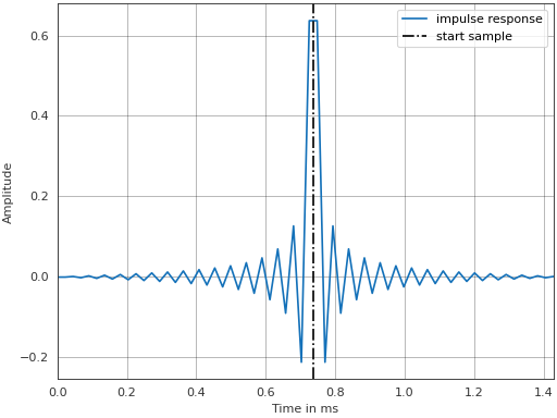
- property invert#
Invert signal using frequency-dependent regularized inversion.
- Returns:
inverse – The inverted signal.
- Return type:
- property regularization#
Regularization \(\epsilon(f)\) without scaling by \(\beta\).
- property signal#
Signal \(S(f)\) to be inverted.
- property target#
Target function \(D(f)\).
- pyfar.dsp.average(signal, mode='linear', caxis=None, weights=None, keepdims=False, nan_policy='raise')[source]#
Average multi-channel signals.
- Parameters:
signal (Signal, TimeData, FrequencyData) – Input signal.
mode (string) –
'linear'Average
signal.timeif the signal is in the time domain andsignal.freqif the signal is in the frequency domain. Note that these operations are equivalent for Signal objects due to the linearity of the averaging and the FFT.'magnitude_zerophase'Average the magnitude spectra and discard the phase.
'magnitude_phase'Average the magnitude spectra and the unwrapped phase separatly.
'power'Average the power spectra \(|X|^2\) and discard the phase. The squaring of the spectra is reversed before returning the averaged signal.
'log_magnitude_zerophase'Average the logarithmic magnitude spectra using
decibeland discard the phase. The logarithm is reversed before returning the averaged signal.
The default is
'linear'caxis (None, int, or tuple of ints, optional) – Channel axes (caxis) along which the averaging is done. The caxis denotes an axis of the data inside an audio object but ignores the last axis that contains the time samples or frequency bins. The default
Noneaverages across all channels.weights (array like) – Array with channel weights for averaging the data. Must be broadcastable to
cshape. The default isNone, which applies equal weights to all channels.keepdims (bool, optional) – If this is
True, the axes which are reduced during the averaging are kept as a dimension with size one. Otherwise, singular dimensions will be squeezed after averaging. The default isFalse.nan_policy (string, optional) –
Define how to handle NaNs in input signal.
'propagate'If the input signal includes NaNs, the corresponding averaged output signal value will be NaN.
'omit'NaNs will be omitted while averaging. For each NaN value, the number of values used for the average operation is also reduced by one. If a signal contains only NaN values in a specific dimensions, the output will be zero. For example if the second sample of a multi channel signal is always NaN, the average will be zero at the second sample.
'raise'A
'ValueError'will be raised, if the input signal includes NaNs.
The default is
'raise'.
- Returns:
averaged_signal – Averaged input Signal.
- Return type:
Notes
The functions
linear_phaseandminimum_phasecan be used to obtain a phase for magnitude spectra after using a mode that discards the phase.
- pyfar.dsp.convolve(signal1, signal2, mode='full', method='overlap_add')[source]#
Convolve two signals.
- Parameters:
signal1 (Signal) – The first signal
signal2 (Signal) – The second signal. The channel shape (cshape) of this signal must be broadcastable to the cshape of the first signal. The cshape gives the shape of the data inside an audio object but ignores the number of samples or frequency bins.
mode (string, optional) –
A string indicating the size of the output:
'full'Compute the full discrete linear convolution of the input signals. The output has the length
'signal1.n_samples + signal2.n_samples - 1'(Default).'cut'Compute the complete convolution with
fulland truncate the result to the length of the longer signal.'cyclic'The output is the cyclic convolution of the signals, where the shorter signal is zero-padded to fit the length of the longer one. This is done by computing the complete convolution with
'full', adding the tail (i.e., the part that is truncated formode='cut'to the beginning of the result) and truncating the result to the length of the longer signal.
method (str {'overlap_add', 'fft'}, optional) –
A string indicating which method to use to calculate the convolution:
'overlap_add'Convolve using the overlap-add algorithm based on
scipy.signal.oaconvolve.. (Default)'fft'Convolve using FFT based on
scipy.signal.fftconvolve.
See Notes for more details.
- Returns:
signal – The result of the convolution. The channel dimension (cdim) matches the bigger cdim of the two input signals. The channel dimension gives the number of dimensions of the audio data excluding the last dimension, which is
n_samplesfor time domain objects andn_binsfor frequency domain objects.- Return type:
Notes
The overlap-add method is generally much faster than fft convolution when one signal is much larger than the other, but can be slower when only a few output values are needed or when the signals have a very similar length. For
method='overlap_add', integer data will be cast to float.Examples
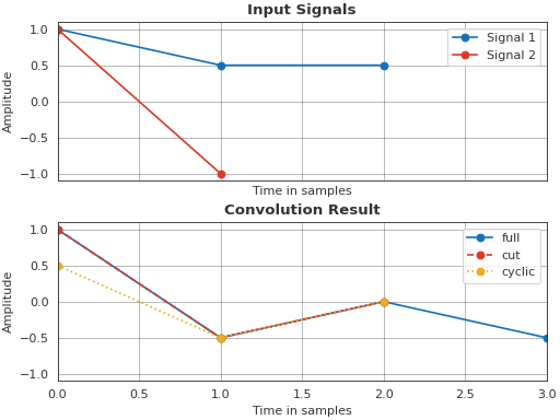
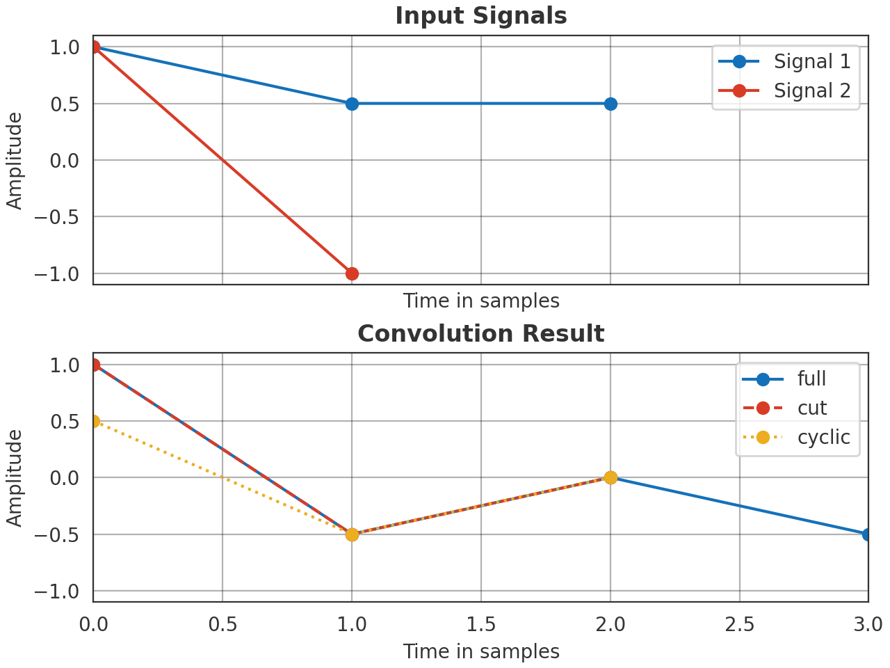
Illustrate the different modes.
>>> import pyfar as pf
>>> s1 = pf.Signal([1, 0.5, 0.5], 1000)
>>> s2 = pf.Signal([1,-1], 1000)
>>> full = pf.dsp.convolve(s1, s2, mode='full')
>>> cut = pf.dsp.convolve(s1, s2, mode='cut')
>>> cyc = pf.dsp.convolve(s1, s2, mode='cyclic')
>>> # Plot input and output
>>> with pf.plot.context():
>>>     fig, ax = plt.subplots(2, 1, sharex=True)
>>>     pf.plot.time(s1, ax=ax[0], label='Signal 1', marker='o',
...                  unit='samples')
>>>     pf.plot.time(s2, ax=ax[0], label='Signal 2', marker='o',
...                  unit='samples')
>>>     ax[0].set_title('Input Signals')
>>>     ax[0].legend()
>>>     pf.plot.time(full, ax=ax[1], label='full', marker='o',
...                  unit='samples')
>>>     pf.plot.time(cut, ax=ax[1], label='cut', ls='--',  marker='o',
...                  unit='samples')
>>>     pf.plot.time(cyc, ax=ax[1], label='cyclic', ls=':', marker='o',
...                  unit='samples')
>>>     ax[1].set_title('Convolution Result')
>>>     ax[1].set_ylim(-1.1, 1.1)
>>>     ax[1].legend()
(
Source code,png,hires.png,pdf)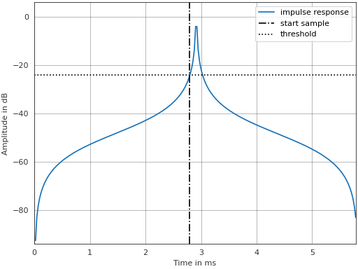
- pyfar.dsp.correlate(signal_1, signal_2, mode='full', normalize=False)[source]#
Compute the channel-wise correlation function between signals.
The correlation function of the time signals \(x_1[n]\) and \(x_2[n]\) is given by
\[c[l] = \sum_n x_1[n] x_2[n-l]\]with the index \(n\) and time lag \(l\) in samples. The computation is realized in the frequency domain using the corresponding spectra \(X_1[k]\) and \(X_2[k]\)
\[c = \mathrm{IFFT\{X_1 X_2^-\}}\]with the inverse fourier transform denoted by IFFT and \(X^-\) denoting the spectrum of a time-reversed and complex conjugated time signal, i.e.,
X_minus = fft(conj(x[::-1]))where the conjugate is required if the input has complex-valued time data.- Parameters:
signal_1 (Signal) – The first input signal. It must have the same sample rate as signal_2 and its
cshapemust be broadcastable to that of signal_2.signal_2 (Signal) – The second input signal. It must have the same sample rate as signal_1 and its
cshapemust be broadcastable to that of signal_1.mode (str, optional) –
Specifies how the correlation is computed.
'full'Computes the full correlation function by zero padding the input signals to a length of
signal_1.n_samples + signal_2.n_samples - 1before applying the Fourier transform (see equations above).'cyclic'Computes the cyclic correlation function, which uses the input signals as they are. In this case signal_1 and signal_2 must have the same number of samples (length).
The default is
'full'.normalize (bool, optional) – If
True, the correlation function is normalized to force \(|c[l]|\leq1\). This is done by the division \(c[l]/\sqrt{E(x_1[n])\,E(x_2[n])}\), where \(E(\cdot)\) denotes theenergy. The defaultFalsedoes not apply any normalization. Normalization is not available for complex-valued time signals.
- Returns:
correlation – The correlation function \(c[l]\) is contained in
correlation.timeand the lags in seconds, i.e., the delays applied to signal_2 (see equations above) are contained incorrelation.times.correlation.timeis complex if one of the input signals has complex-valued time data. The cshape of correlation matches the cshape to which signal_1 and signal_2 were broadcasted. The lags can be converted to samples by multiplication withsignal_1.sampling_rate. In this case, they are in the interval[-signal_2.n_samples + 1, signal_1.n_samples - 1]if the full correlation was computed. In case of the cyclic correlation, they are in the interval[-(signal_1.n_samples // 2) + 1, signal_1.n_samples // 2]if the signals have an even number of samples, and in the interval[-(signal_1.n_samples // 2), signal_1.n_samples // 2]if the signals have an odd number of samples.- Return type:
Examples
Compute the lags (delay) that are required to maximize the cross-correlation between a one and multi-dimensional signal
>>> import pyfar as pf
>>> import numpy as np
>>>
>>> # one-dimensional signal: impulse with zero delay
>>> signal_1 = pf.signals.impulse(5, 0)
>>>
>>> # multi-dimension signal with cshape = (2, 2):
>>> # impulses with non-zero delays
>>> delays = np.array([[0, 1], [2, 3]], dtype=int)
>>> signal_2 = pf.signals.impulse(5, delays)
>>>
>>> cor = pf.dsp.correlate(signal_1, signal_2, 'full')
>>>
>>> # compute the lags in samples
>>> argmax = cor.times[np.argmax(cor.time, axis=-1)]
>>>
>>> # plot correlation and indicate maximum
>>> ax = pf.plot.time(cor, unit='ms')
>>> ax.set_title('Correlation and position of maxima (dots)')
>>> ax.set_xlabel('Time lag in ms')
>>> ax.set_ylabel('Auto correlation')
>>> for amax, color in zip(argmax.flatten(), 'bryp'):
>>>     ax.axvline(amax, color=pf.plot.color(color), linestyle=':')
(
Source code,png,hires.png,pdf)
Linear and cyclic auto-correlation of a perfect sequence. Perfect sequences have unit auto-correlation for \(l=0\) and zero auto-correlation otherwise
>>> import pyfar as pf
>>>
>>> signal = pf.signals.linear_perfect_sweep(2**7)
>>>
>>> for mode in ['full', 'cyclic']:
>>>     line = '--' if mode == 'cyclic' else '-'
>>>     cor = pf.dsp.correlate(signal, signal, mode, normalize=True)
>>>     ax = pf.plot.time(cor, unit='ms', label=mode, ls=line)
>>>
>>> ax.set_xlabel('Time lag in ms')
>>> ax.set_ylabel('Auto correlation')
>>> ax.legend()
(
Source code,png,hires.png,pdf)
- pyfar.dsp.decibel(signal, domain='freq', log_prefix=None, log_reference=1, return_prefix=False)[source]#
Convert data of the selected signal domain into decibels (dB).
The converted data is calculated by the base 10 logarithmic scale:
data_in_dB = log_prefix * numpy.log10(data/log_reference). By using a logarithmic scale, the deciBel is able to compare quantities that may have vast ratios between them. As an example, the sound pressure in dB can be calculated as followed:\[L_p = 20\log_{10}\biggl(\frac{p}{p_0}\biggr),\]where \(20\) is the logarithmic prefix for sound field quantities and \(p_0\) would be the reference for the sound pressure level. A list of commonly used reference values can be found in the ‘log_reference’ parameters section.
- Parameters:
signal (Signal, TimeData, FrequencyData) – The signal which is converted into decibel
domain (str) –
The domain, that is converted to decibels:
'freq'Convert normalized frequency domain data. Signal must be of type ‘Signal’ or ‘FrequencyData’.
'time'Convert time domain data. Signal must be of type ‘Signal’ or ‘TimeData’.
'freq_raw'Convert frequency domain data without normalization. Signal must be of type ‘Signal’.
The default is
'freq'.log_prefix (int) – The prefix for the dB calculation. The default
None, uses10for signals with'psd'and'power'FFT normalization and20otherwise.log_reference (int or float) –
Reference for the logarithm calculation. List of commonly used values:
log_reference
value
Digital signals (dBFs)
1
Sound pressure \(L_p\) (dB)
2e-5 Pa
Voltage \(L_V\) (dBu)
0.7746 volt
Sound intensity \(L_I\) (dB)
1e-12 W/m²
Voltage \(L_V\) (dBV)
1 volt
Electric power \(L_P\) (dB)
1 watt
The default is 1.
return_prefix (bool, optional) – If return_prefix is
True, the function will also return the log_prefix value. This can be used to delogrithmize the data. The default isFalse.
- Returns:
decibel (numpy.ndarray) – The given signal in decibel in chosen domain.
log_prefix (int or float) – Will be returned if return_prefix is set to
True.
Examples
>>> import pyfar as pf
>>> signal = pf.signals.noise(41000, rms=[1, 1])
>>> decibel_data = decibel(signal, domain='time')
- pyfar.dsp.deconvolve(system_output, system_input, fft_length=None, frequency_range=None, **kwargs)[source]#
Calculate transfer functions by spectral deconvolution of two signals.
Note
This function will be deprecated in pyfar v0.10.0 in favor of
pyfar.dsp.RegularizedSpectrumInversionandpyfar.dsp.convolve.The transfer function \(H(\omega)\) is calculated by spectral deconvolution (spectral division).
\[H(\omega) = \frac{Y(\omega)}{X(\omega)},\]where \(X(\omega)\) is the system input signal and \(Y(\omega)\) the system output. Regularized inversion is used to avoid numerical issues in calculating \(X(\omega)^{-1} = 1/X(\omega)\) for small values of \(X(\omega)\) (see
regularized_spectrum_inversion). The system response (transfer function) is thus calculated as\[H(\omega) = Y(\omega)X(\omega)^{-1}.\]For more information, refer to [2].
- Parameters:
system_output (Signal) – The system output signal (e.g., recorded after passing a device under test). The system output signal is zero padded, if it is shorter than the system input signal.
system_input (Signal) – The system input signal (e.g., used to perform a measurement). The system input signal is zero padded, if it is shorter than the system output signal.
frequency_range (tuple, array_like, double) – The upper and lower frequency limits outside of which the regularization factor is to be applied. The default
Nonebypasses the regularization, which might cause numerical instabilities in case of band-limited system_input. Also seeregularized_spectrum_inversion.fft_length (int or None) – The length the signals system_output and system_input are zero padded to before deconvolving. The default is None. In this case only the shorter signal is padded to the length of the longer signal, no padding is applied when both signals have the same length.
kwargs (key value arguments) – Key value arguments to control the inversion of \(H(\omega)\) are passed to to
regularized_spectrum_inversion.
- Returns:
system_response – The resulting signal after deconvolution, representing the system response (the transfer function). The
fft_normof is set to'none'.- Return type:
References
- pyfar.dsp.energy(signal)[source]#
Computes the channel wise energy in the time domain.
\[\sum_{n=0}^{N-1}|x[n]|^2=\frac{1}{N}\sum_{k=0}^{N-1}|X[k]|^2,\]which is equivalent to the frequency domain computation according to Parseval’s theorem [3].
- Parameters:
signal (Signal) – The signal to compute the energy from.
- Returns:
data – The channel-wise energy of the input signal.
- Return type:
Notes
Due to the calculation based on the time data, the returned energy is independent of the signal’s
fft_norm.powerandrmscan be used to compute the power and the rms of a signal.References
- pyfar.dsp.find_impulse_response_delay(impulse_response, N=1)[source]#
Find the delay in sub-sample values of an impulse response.
The method relies on the analytic part of the cross-correlation function of the impulse response and it’s minimum-phase equivalent, which is zero for the maximum of the correlation function. For sub-sample root finding, the analytic signal is approximated using a polynomial of order
N. The algorithm is based on [4] with the following modifications:Values with negative gradient used for polynomial fitting are rejected, allowing to use larger part of the signal for fitting.
By default a first order polynomial is used, as the slope of the analytic signal should in theory be linear.
Alternatively see
pyfar.dsp.find_impulse_response_start. For complex-valued time signals, the delay is calculated separately for the real and complex part, and its minimum value returned.- Parameters:
impulse_response (Signal) – The impulse response.
N (int, optional) – The order of the polynom used for root finding, by default 1.
- Returns:
delay – Delay of the impulse response, as an array of shape
cshape. Can be floating point values in the case of sub-sample values.- Return type:
numpy.ndarray, float
References
Examples
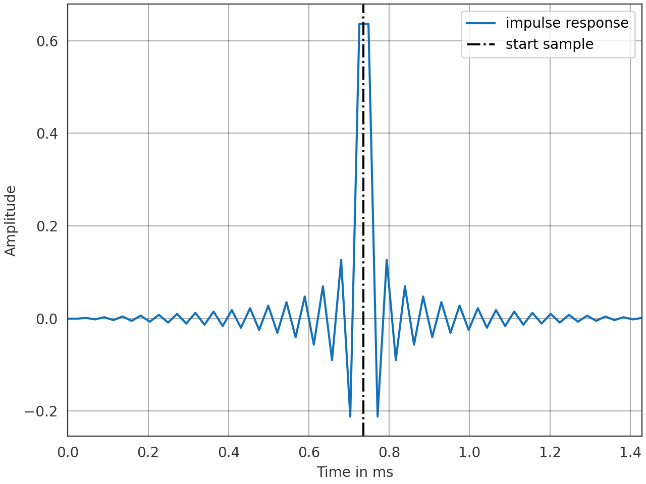
Create a band-limited impulse shifted by 0.5 samples and estimate the starting sample of the impulse and plot.
>>> import pyfar as pf
>>> import numpy as np
>>> n_samples = 64
>>> delay_samples = n_samples // 2 + 1/2
>>> ir = pf.signals.impulse(n_samples)
>>> ir = pf.dsp.linear_phase(ir, delay_samples, unit='samples')
>>> start_samples = pf.dsp.find_impulse_response_delay(ir)
>>> ax = pf.plot.time(ir, unit='ms', label='impulse response')
>>> ax.axvline(
...     start_samples/ir.sampling_rate*1e3,
...     color='k', linestyle='-.', label='start sample')
>>> ax.legend()
(
Source code,png,hires.png,pdf)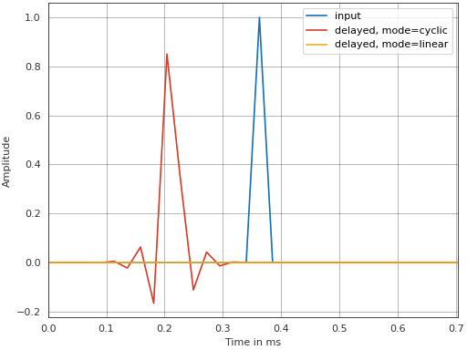
- pyfar.dsp.find_impulse_response_start(impulse_response, threshold=20)[source]#
Find the start sample of an impulse response.
The start sample is identified as the first sample which is below the
thresholdlevel relative to the maximum level of the impulse response. For room impulse responses, ISO 3382 [5] specifies a threshold of 20 dB. This function is primary intended to be used when processing room impulse responses. For complex-valued time signals the onset is computed separately for the real and imaginary part. Alternatively seepyfar.dsp.find_impulse_response_delay.- Parameters:
impulse_response (pyfar.Signal) – The impulse response
threshold (float, optional) – The threshold level in dB, by default 20, which complies with ISO 3382.
- Returns:
start_sample – Sample at which the impulse response starts
- Return type:
numpy.ndarray, int
Notes
The function tries to estimate the PSNR in the IR based on the signal power in the last 10 percent of the IR. The automatic estimation may fail if the noise spectrum is not white or the impulse response contains non-linear distortions. If the PSNR is lower than the specified threshold, the function will issue a warning.
References
Examples
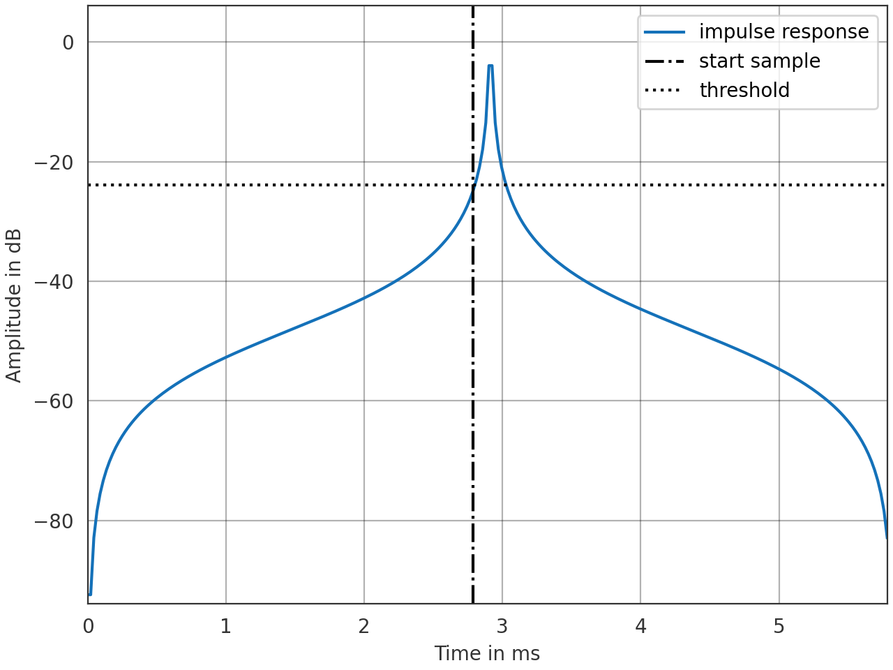
Create a band-limited impulse shifted by 0.5 samples and estimate the starting sample of the impulse and plot.
>>> import pyfar as pf
>>> import numpy as np
>>> n_samples = 256
>>> delay_samples = n_samples // 2 + 1/2
>>> ir = pf.signals.impulse(n_samples)
>>> ir = pf.dsp.linear_phase(ir, delay_samples, unit='samples')
>>> start_samples = pf.dsp.find_impulse_response_start(ir)
>>> ax = pf.plot.time(ir, unit='ms', label='impulse response', dB=True)
>>> ax.axvline(
...     start_samples/ir.sampling_rate*1e3,
...     color='k', linestyle='-.', label='start sample')
>>> ax.axhline(
...     20*np.log10(np.max(np.abs(ir.time)))-20,
...     color='k', linestyle=':', label='threshold')
>>> ax.legend()
(
Source code,png,hires.png,pdf)
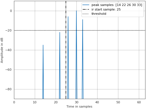
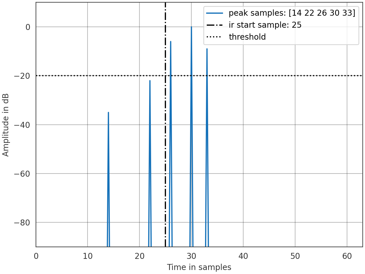
Create a train of weighted impulses with levels below and above the threshold, serving as a very abstract room impulse response. The starting sample is identified as the last sample below the threshold relative to the maximum of the impulse response.
>>> import pyfar as pf
>>> import numpy as np
>>> n_samples = 64
>>> delays = np.array([14, 22, 26, 30, 33])
>>> amplitudes = np.array([-35, -22, -6, 0, -9], dtype=float)
>>> ir = pf.signals.impulse(n_samples, delays, 10**(amplitudes/20))
>>> ir.time = np.sum(ir.time, axis=0)
>>> start_sample_est = pf.dsp.find_impulse_response_start(
...     ir, threshold=20)
>>> ax = pf.plot.time(
...     ir, dB=True, unit='samples',
...     label=f'peak samples: {delays}')
>>> ax.axvline(
...     start_sample_est, linestyle='-.', color='k',
...     label=f'ir start sample: {start_sample_est}')
>>> ax.axhline(
...     20*np.log10(np.max(np.abs(ir.time)))-20,
...     color='k', linestyle=':', label='threshold')
>>> ax.legend()
(
Source code,png,hires.png,pdf)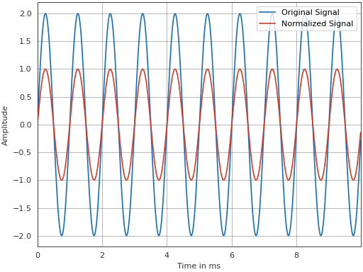
- pyfar.dsp.fractional_time_shift(signal, shift, unit='samples', order=30, side_lobe_suppression=60, mode='linear')[source]#
Apply fractional time shift to input data.
This function uses a windowed Sinc filter (Method FIR-2 in [6] according to Equations 21 and 22) to apply fractional delays, i.e., non-integer delays to an input signal. A Kaiser window according to [7] Equations (10.12) and (10.13) is used, which offers the possibility to control the side lobe suppression.
- Parameters:
signal (Signal) – The input data
shift (float, array like) – The fractional shift in samples (positive or negative). If this is a float, the same shift is applied to all channels of signal. If this is an array like different delays are applied to the channels of signal. In this case it must broadcast to signal.cshape (see Numpy broadcasting)
unit (str, optional) – The unit of the shift. Either ‘samples’ or ‘s’. Defaults to ‘samples’.
order (int, optional) – The order of the fractional shift (sinc) filter. The precision of the filter increases with the order. High frequency errors decrease with increasing order. The order must be smaller than
signal.n_samples. The default is30.side_lobe_suppression (float, optional) – The side lobe suppression of the Kaiser window in dB. The default is
60.mode (str, optional) –
The filtering mode
"linear"Apply linear shift, i.e., parts of the signal that are shifted to times smaller than 0 samples and larger than
signal.n_samplesdisappear."cyclic"Apply a cyclic shift, i.e., parts of the signal that are shifted to values smaller than 0 are wrapped around to the end, and parts that are shifted to values larger than
signal.n_samplesare wrapped around to the beginning.
The default is
"linear"
- Returns:
signal – The delayed input data
- Return type:
References
Examples
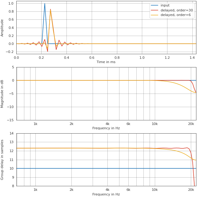
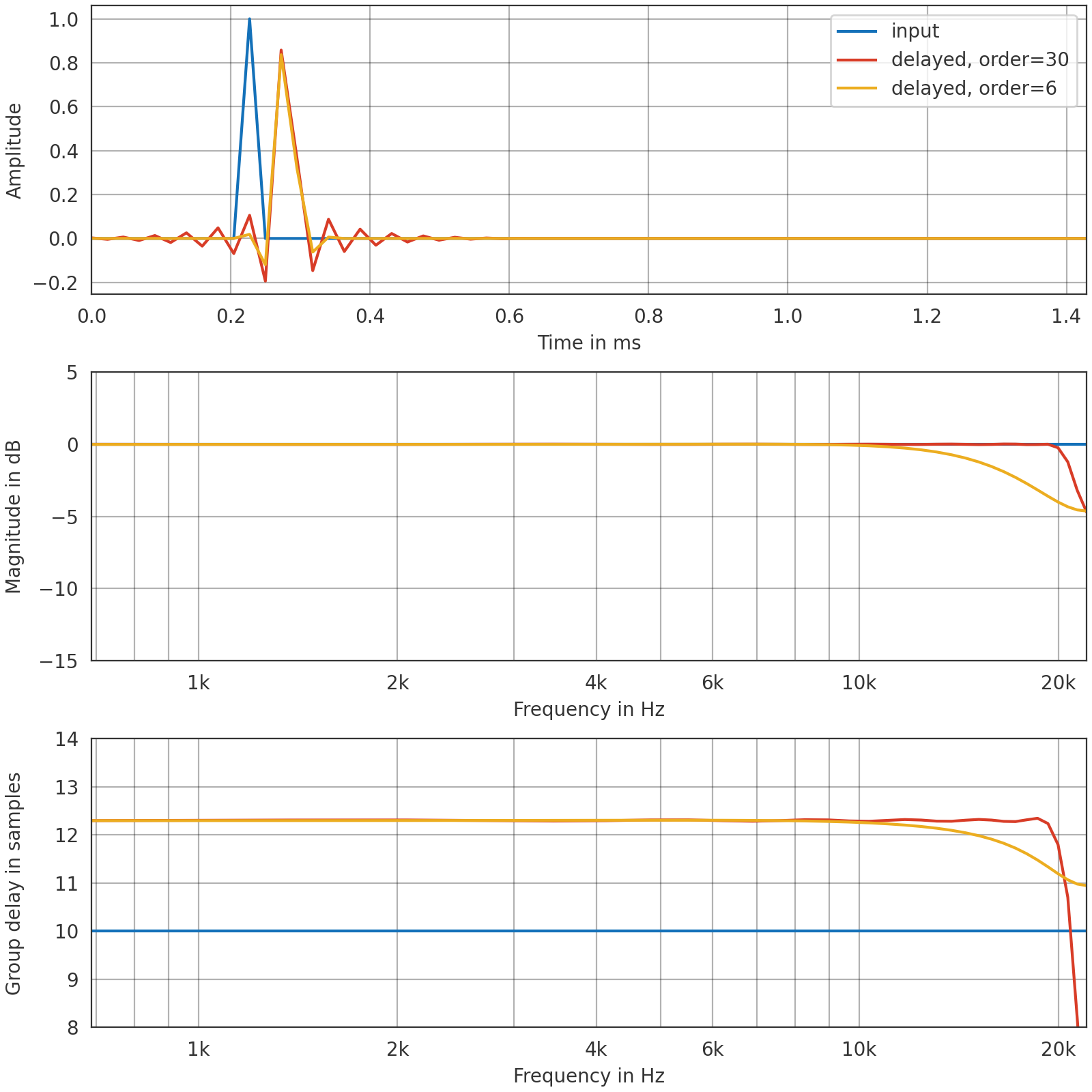
Apply a fractional shift of 2.3 samples using filters of orders 6 and 30
>>> import pyfar as pf
>>> import matplotlib.pyplot as plt
>>>
>>> signal = pf.signals.impulse(64, 10)
>>>
>>> pf.plot.use()
>>> _, ax = plt.subplots(3, 1, figsize=(8, 8))
>>> pf.plot.time_freq(signal, ax=ax[:2], label="input", unit='ms')
>>> pf.plot.group_delay(signal, ax=ax[2], unit="samples")
>>>
>>> for order in [30, 6]:
>>>     delayed = pf.dsp.fractional_time_shift(
...         signal, 2.3, order=order)
>>>     pf.plot.time_freq(delayed, ax=ax[:2],
...                       label=f"delayed, order={order}", unit='ms')
>>>     pf.plot.group_delay(delayed, ax=ax[2], unit="samples")
>>>
>>> ax[1].set_ylim(-15, 5)
>>> ax[2].set_ylim(8, 14)
>>> ax[0].legend()
(
Source code,png,hires.png,pdf)
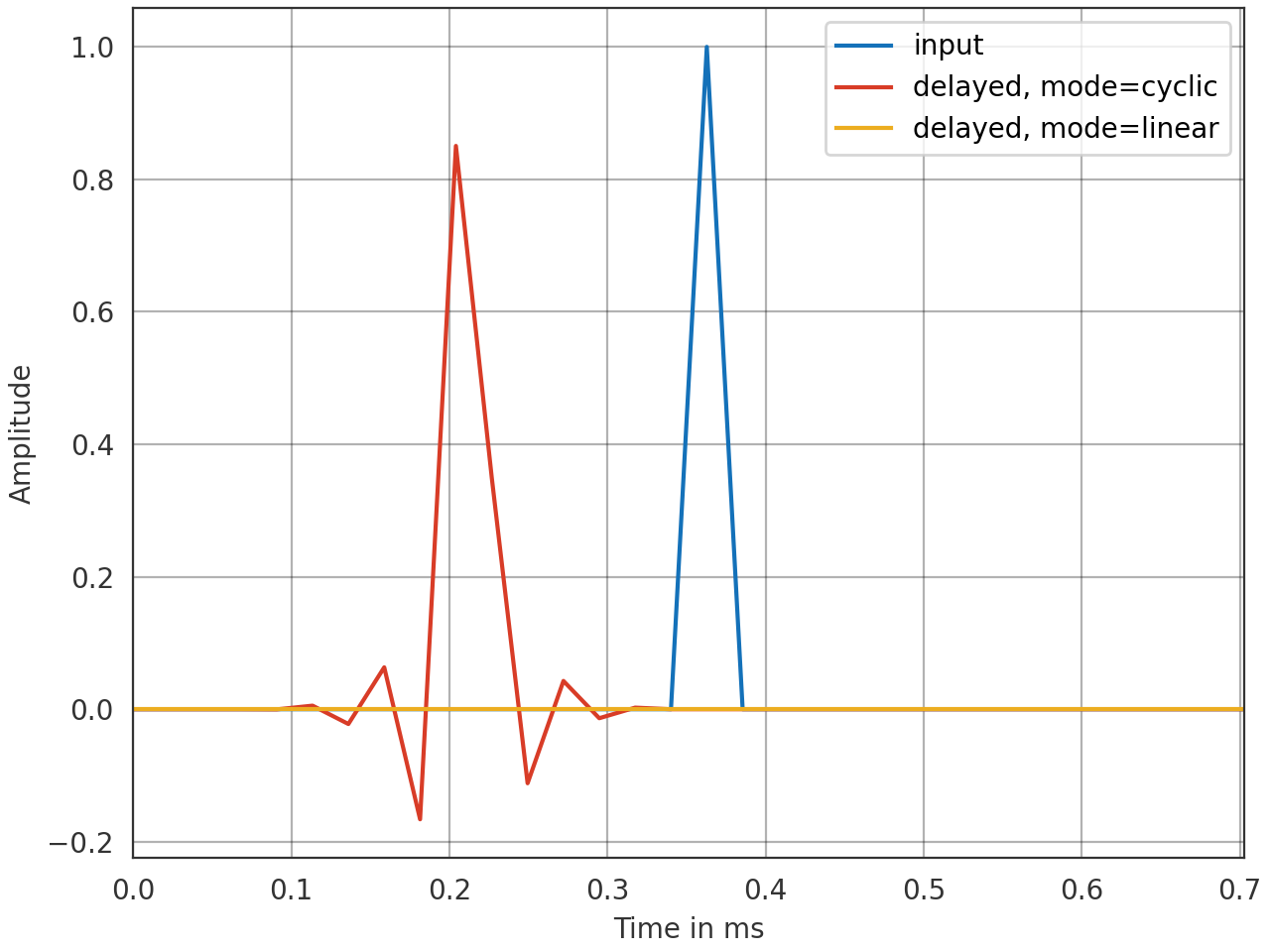
Apply a shift that exceeds the signal length using the modes
"linear"and"cyclic">>> import pyfar as pf >>> >>> signal = pf.signals.impulse(32, 16) >>> >>> ax = pf.plot.time(signal, label="input", unit='ms') >>> >>> for mode in ["cyclic", "linear"]: >>> delayed = pf.dsp.fractional_time_shift( ... signal, 25.3, order=10, mode=mode) >>> pf.plot.time(delayed, label=f"delayed, mode={mode}", unit='ms') >>> >>> ax.legend()
(
Source code,png,hires.png,pdf)
- pyfar.dsp.group_delay(signal, frequencies=None, method='fft')[source]#
Returns the group delay of a signal in samples.
- Parameters:
signal (Signal) – An audio signal object from the pyfar signal class
frequencies (array-like) – Frequency or frequencies in Hz at which the group delay is calculated. The default is
None, in which case signal.frequencies is used.method ('scipy', 'fft', optional) – Method to calculate the group delay of a Signal. Both methods calculate the group delay using the method presented in [8] avoiding issues due to discontinuities in the unwrapped phase. Note that the scipy version additionally allows to specify frequencies for which the group delay is evaluated. The default is
'fft', which is faster.
- Returns:
group_delay – Frequency dependent group delay of shape (
cshape, frequencies).- Return type:
numpy array
References
- pyfar.dsp.kaiser_window_beta(A)[source]#
Return a shape parameter beta to create kaiser window based on desired side lobe suppression in dB.
This function can be used to call
time_windowwithwindow=('kaiser', beta).- Parameters:
A (float) – Side lobe suppression in dB
- Returns:
beta – Shape parameter beta after [9], Eq. 7.75
- Return type:
float
References
- pyfar.dsp.linear_phase(signal, group_delay, unit='samples')[source]#
Set the phase to a linear phase with a specified group delay.
The linear phase signal is computed as
\[H_{\mathrm{lin}} = |H| \mathrm{e}^{-j \omega \tau}\,,\]with \(H\) the complex spectrum of the input data, \(|\cdot|\) the absolute values, \(\omega\) the frequency in radians and \(\tau\) the group delay in seconds.
- Parameters:
signal (Signal) – input data
group_delay (float, array like) – The desired group delay of the linear phase signal according to unit. A reasonable value for most cases is
signal.n_samples / 2samples, which results in a time signal that is symmetric around the center. If group delay is a list or array it must broadcast with the channel layout of the signal (signal.cshape).unit (string, optional) – Unit of the group delay. Can be
'samples'or's'for seconds. The default is'samples'.
- Returns:
signal – linear phase copy of the input data
- Return type:
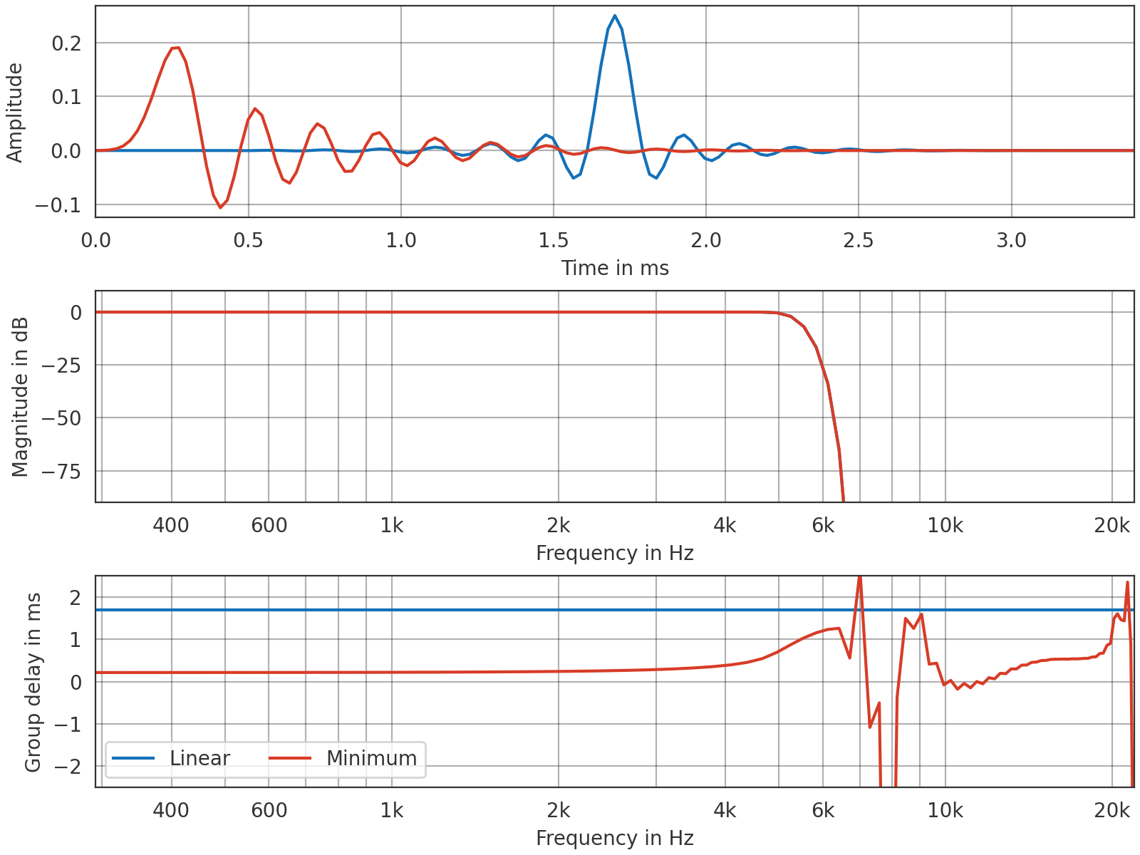
- pyfar.dsp.minimum_phase(signal, n_fft=None, truncate=True)[source]#
Calculate the minimum phase equivalent of a finite impulse response.
The method is based on the Hilbert transform of the real-valued cepstrum of the finite impulse response, that is the cepstrum of the magnitude spectrum only. As a result the magnitude spectrum is not distorted. Potential aliasing errors can occur due to the Fourier transform based calculation of the magnitude spectrum, which however are negligible if the length of Fourier transform
n_fftis sufficiently high. [10] (Section 8.5.4)- Parameters:
signal (Signal) – The finite impulse response for which the minimum-phase version is computed.
n_fft (int, optional) – The FFT length used for calculating the cepstrum. Should be at least a few times larger than
signal.n_samples. The defaultNoneuses eight times the signal length rounded up to the next power of two, that is:2**int(np.ceil(np.log2(n_samples * 8))).truncate (bool, optional) – If
truncateisTrue, the resulting minimum phase impulse response is truncated to a length ofsignal.n_samples//2 + signal.n_samples % 2. This avoids aliasing described above in any case but might distort the magnitude response ifsignal.n_samplesis too low. If truncate isFalsethe output signal has the same length as the input signal. The default isTrue.
- Returns:
signal_minphase – The minimum phase version of the input data.
- Return type:
References
Examples
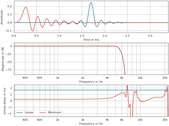
Create a minimum phase equivalent of a linear phase FIR low-pass filter
>>> import pyfar as pf
>>> import numpy as np
>>> from scipy.signal import remez
>>> import matplotlib.pyplot as plt
>>> freq = [0, 0.2, 0.3, 1.0]
>>> h_linear = pf.Signal(remez(151, freq, [1, 0], fs=2.), 44100)
>>> # create minimum phase impulse responses
>>> h_min = pf.dsp.minimum_phase(h_linear, truncate=False)
>>> # plot the result
>>> pf.plot.use()
>>> fig, axs = plt.subplots(3, figsize=(8, 6))
>>> pf.plot.time(h_linear, ax=axs[0], unit='ms')
>>> pf.plot.time(h_min, ax=axs[0], unit='ms')
>>> axs[0].grid(True)
>>> pf.plot.freq(h_linear, ax=axs[1])
>>> pf.plot.group_delay(h_linear, ax=axs[2], unit="ms")
>>> pf.plot.freq(h_min, ax=axs[1])
>>> pf.plot.group_delay(h_min, ax=axs[2], unit="ms")
>>> axs[2].legend(['Linear', 'Minimum'], loc=3, ncol=2)
>>> axs[2].set_ylim(-2.5, 2.5)
(
Source code,png,hires.png,pdf)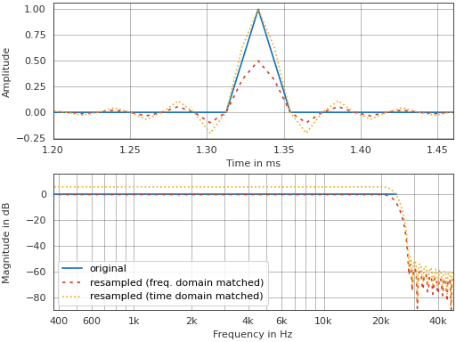
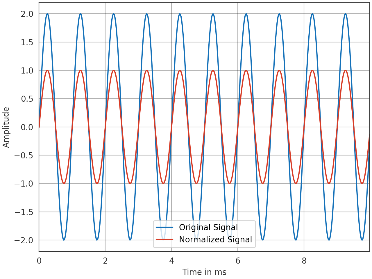
- pyfar.dsp.normalize(signal, reference_method='max', domain='auto', channel_handling='individual', target=1, limits=(None, None), unit=None, return_reference=False, nan_policy='raise')[source]#
Apply a normalization.
In the default case, the normalization ensures that the maximum absolute amplitude of the signal after normalization is 1. This is achieved by the multiplication
signal_normalized = signal * target / reference,where target equals 1 and reference is the maximum absolute amplitude before the normalization.
Several normalizations are possible, which in fact are different ways of computing the reference value (e.g. based on the spectrum). See the parameters for details.
- Parameters:
signal (Signal, TimeData, FrequencyData) – Input signal.
reference_method (string, optional) –
Reference method to compute the channel-wise reference value using the data according to domain.
'max'Compute the maximum absolute value per channel.
'mean'Compute the mean absolute values per channel.
'energy'Compute the energy per channel using
energy. Note that the square root of the energy is used as reference, after handling multi-channel signals (see channel_handling below). This is required for the energy of the normalized signal to match the target.'power'Compute the power per channel using
power. Note that the square root of the power is used as reference, after handling multi-channel signals (see channel_handling below). This is required for the power of the normalized signal to match the target.'rms'Compute the RMS per channel using
rms.
The default is
'max'.domain (string) –
Determines which data is used to compute the reference value.
'time'Use the absolute of the time domain data
np.abs(signal.time).'freq'Use the magnitude spectrum
np.abs(signal.freq). Note that the normalized magnitude spectrum is used pyfar examples gallery (cf. FFT normalization).'auto'Uses
'time'domain normalization forSignalandTimeDataobjects and'freq'domain normalization forFrequencyDataobjects.
The default is
'auto'.channel_handling (string, optional) –
- Define how channel-wise reference values are handeled for multi-
channel signals. This parameter does not affect single-channel signals.
'individual'Separate normalization of each channel individually.
'max'Normalize to the maximum reference value across channels.
'min'Normalize to the minimum reference value across channels.
'mean'Normalize to the mean reference value across the channels.
The default is
'individual'.target (scalar, array) – The target to which the signal is normalized. Can be a scalar or an array. In the latter case the shape of target must be broadcastable to
cshape. The default is1.limits (tuple, array_like) – Restrict the time or frequency range that is used to compute the reference value. Two element tuple specifying upper and lower limit according to domain and unit. A None element means no upper or lower limitation. The default
(None, None)uses the entire signal. Note that in case of limiting in samples or bins withunit=None, the second value defines the first sample/bin that is excluded. Also note that limits need to be(None, None)if reference_method isrms,powerorenergy.unit (string, optional) –
Unit of limits.
's'Set limits in seconds in case of time domain normalization. Uses
find_nearest_timeto find the limits.'Hz'Set limits in hertz in case of frequency domain normalization. Uses
find_nearest_frequency
The default
Noneassumes that limits is given in samples in case of time domain normalization and in bins in case of frequency domain normalization.return_reference (bool) – If
return_reference=True, the function also returns the reference values for the channels. The default isFalse.nan_policy (string, optional) –
Define how to handle NaNs in input signal.
'propagate'If the input signal includes NaNs within the time or frequency range , NaN will be used as normalization reference. The resulting output signal values are NaN.
'omit'NaNs will be omitted in the normalization. Cshape will still remain, as the normalized signal still includes the NaNs.
'raise'A
ValueErrorwill be raised, if the input signal includes NaNs.
The default is ‘raise’.
- Returns:
normalized_signal (Signal, TimeData, FrequencyData) – The normalized input signal.
reference_norm (numpy.ndarray) – The reference values used for normalization. Only returned if return_reference is
True.
Examples
Time domain normalization with default parameters
>>> import pyfar as pf
>>> signal = pf.signals.sine(1e3, 441, amplitude=2)
>>> signal_norm = pf.dsp.normalize(signal)
>>> # Plot input and normalized Signal
>>> ax = pf.plot.time(signal, label='Original Signal', unit='ms')
>>> pf.plot.time(signal_norm, label='Normalized Signal', unit='ms')
>>> ax.legend()
(
Source code,png,hires.png,pdf)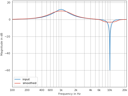
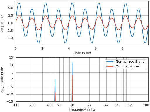
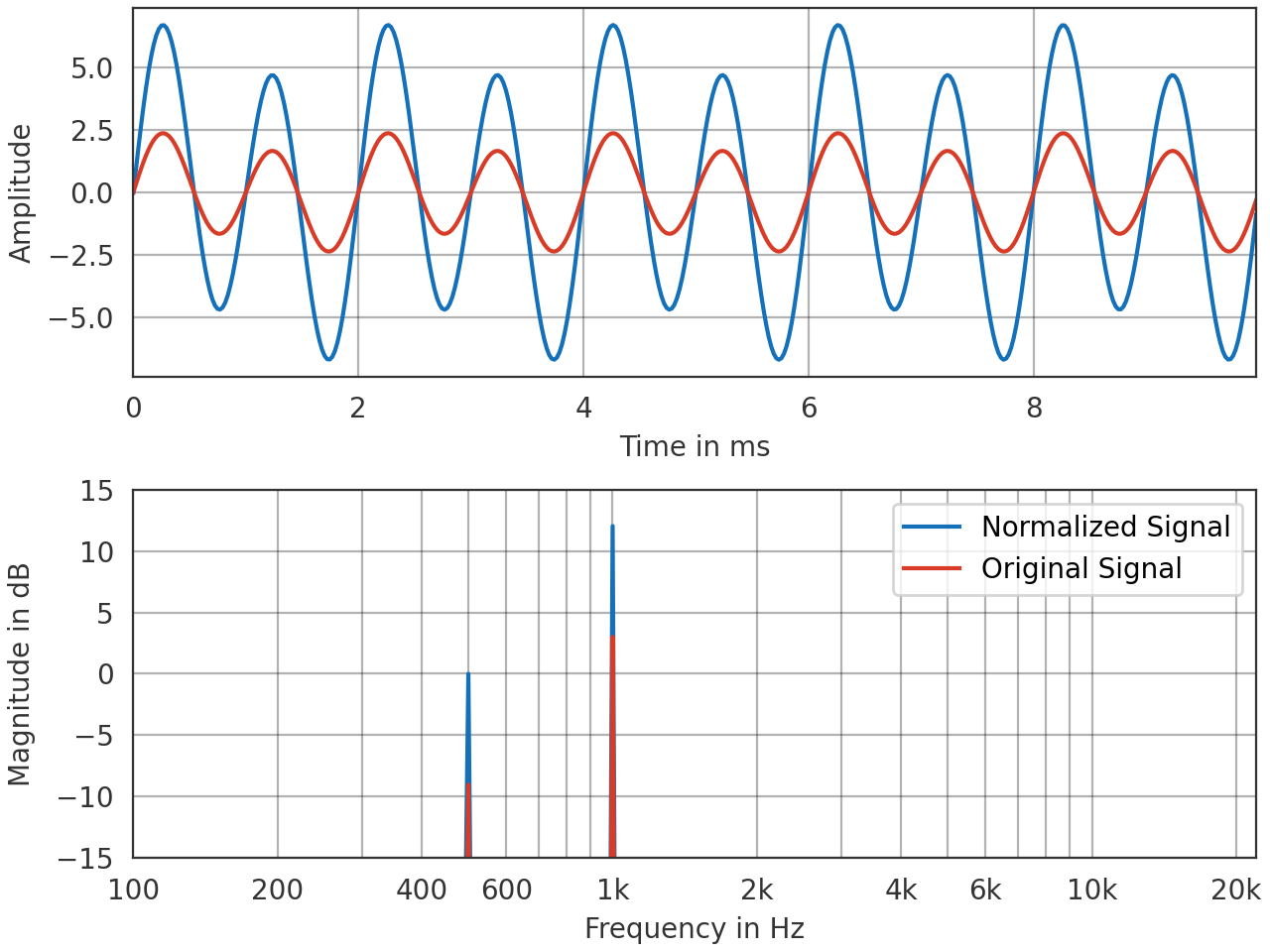
Frequency normalization with a restricted frequency range and targed in dB
>>> import pyfar as pf
>>> sine1 = pf.signals.sine(1e3, 441, amplitude=2)
>>> sine2 = pf.signals.sine(5e2, 441, amplitude=.5)
>>> signal = sine1 + sine2
>>> # Normalize to dB target in restricted frequency range
>>> target_dB = 0
>>> signal_norm = pf.dsp.normalize(signal, target=10**(target_dB/20),
...     domain="freq", limits=(400, 600), unit="Hz")
>>> # Plot input and normalized Signal
>>> ax = pf.plot.time_freq(signal_norm, label='Normalized Signal',
...                        unit='ms')
>>> pf.plot.time_freq(signal, label='Original Signal', unit='ms')
>>> ax[1].set_ylim(-15, 15)
>>> ax[1].legend()
(
Source code,png,hires.png,pdf)
- pyfar.dsp.pad_zeros(signal, pad_width, mode='end')[source]#
Pad a signal with zeros in the time domain.
- Parameters:
signal (Signal) – The signal which is to be extended.
pad_width (int) – The number of samples to be padded.
mode (str, optional) –
The padding mode:
'end'Append zeros to the end of the signal
'beginning'Prepend zeros to the beginning of the signal
'center'Insert the number of zeros in the middle of the signal. This mode can be used to pad signals with a symmetry with respect to the time
t=0.
The default is
'end'.
- Returns:
The zero-padded signal.
- Return type:
Examples
>>> import pyfar as pf
>>> impulse = pf.signals.impulse(512, amplitude=1)
>>> impulse_padded = pf.dsp.pad_zeros(impulse, 128, mode='end')
- pyfar.dsp.phase(signal, deg=False, unwrap=False)[source]#
Returns the phase for a given signal object.
- Parameters:
signal (Signal, FrequencyData) – pyfar Signal or FrequencyData object.
deg (Boolean) – Specifies, whether the phase is returned in degrees or radians.
unwrap (Boolean) – Specifies, whether the phase is unwrapped or not. If set to
'360', the phase is wrapped to 2 pi.
- Returns:
phase – The phase of the signal.
- Return type:
numpy array
- pyfar.dsp.power(signal)[source]#
Compute the power of a signal.
The power is calculated as
\[\frac{1}{N}\sum_{n=0}^{N-1}|x[n]|^2\]based on the time data for each channel separately.
- Parameters:
signal (Signal) – The signal to compute the power from.
- Returns:
data – The channel-wise power of the input signal.
- Return type:
Notes
Due to the calculation based on the time data, the returned power is independent of the signal’s
fft_norm. The power equals the squared RMS of a signal.energyandrmscan be used to compute the energy and the RMS.
- pyfar.dsp.regularized_spectrum_inversion(signal, frequency_range, regu_outside=1.0, regu_inside=1e-10, regu_final=None, normalized=True)[source]#
Invert the spectrum of a signal applying frequency dependent regularization.
Regularization can either be specified within a given frequency range using two different regularization factors, or for each frequency individually using the parameter regu_final. In the first case the regularization factors for the frequency regions are cross-faded using a raised cosine window function with a width of \(\sqrt{2}f\) above and below the given frequency range. Note that the resulting regularization function is adjusted to the quadratic maximum of the given signal. In case the regu_final parameter is used, all remaining options are ignored and an array matching the number of frequency bins of the signal needs to be given. In this case, no normalization of the regularization function is applied.
Finally, the inverse spectrum is calculated as [11], [12],
\[S^{-1}(f) = \frac{S^*(f)}{S^*(f)S(f) + \epsilon(f)}\]- Parameters:
signal (Signal) – The signals which spectra are to be inverted.
frequency_range (tuple, array_like, double) – The upper and lower frequency limits outside of which the regularization factor is to be applied.
regu_outside (float, optional) – The normalized regularization factor outside the frequency range. The default is
1.regu_inside (float, optional) – The normalized regularization factor inside the frequency range. The default is
10**(-200/20)(-200 dB).regu_final (float, array_like, optional) – The final regularization factor for each frequency, default
None. If this parameter is set, the remaining regularization factors are ignored.normalized (bool) – Flag to indicate if the normalized spectrum (according to signal.fft_norm) should be inverted. The default is
True.
- Returns:
The resulting signal after inversion.
- Return type:
References
- pyfar.dsp.resample(signal, sampling_rate, match_amplitude='auto', frac_limit=None, post_filter=False)[source]#
Resample signal to new sampling rate.
The SciPy function
scipy.signal.resample_polyis used for resampling. The resampling ratioL = sampling_rate/signal.sampling_rateis approximated by a fraction of two integer numbers up/down to first upsample the signal by up and then downsample by down. This way up and down are smaller than the respective new and old sampling rates.Note
sampling_rate should be divisible by 10, otherwise it can cause an infinite loop in the
resample_polyfunction.The amplitudes of the resampled signal can match the amplitude of the input signal in the time or frequency domain. See the parameter match_amplitude and the examples for more information.
- Parameters:
signal (Signal) – Input data to be resampled
sampling_rate (number) – The new sampling rate in Hz
match_amplitude (string) –
Define the domain to match the amplitude of the resampled data.
'auto'Chooses domain to maintain the amplitude automatically, depending on the
signal.signal_type. Setsmatch_amplitude == 'freq'forsignal.signal_type = 'energy'like impulse responses andmatch_amplitude == 'time'for other signals.'time'Maintains the amplitude in the time domain. This is useful for recordings such as speech or music and must be used if
signal.signal_type = 'power'.'freq'Maintains the amplitude in the frequency domain by multiplying the resampled signal by
1/L(see above). This is often desired when resampling impulse responses.
The default is
'auto'.frac_limit (int) –
Limit the denominator for approximating the resampling factor L (see above). This can be used in case the resampling gets stuck in an infinite loop (see note above) at the potenital cost of not exactly realizing the target sampling rate.
The default is
None, which usesfrac_limit = 1e6.post_filter (bool, optional) – In some cases the up-sampling causes artifacts above the Nyquist frequency of the input signal, i.e.,
signal.sampling_rate/2. IfTruethe artifacts are suppressed by applying a zero-phase Elliptic filter with a pass band ripple of 0.1 dB, a stop band attenuation of 60 dB. The pass band edge frequency issignal.sampling_rate/2. The stop band edge frequency is the minimum of 1.05 times the pass band frequency and the new Nyquist frequency (sampling_rate/2). The default isFalse. Note that this is only applied in case of up-sampling.
- Returns:
signal – The resampled signal of the input data with a length of up/down * signal.n_samples samples.
- Return type:
Examples
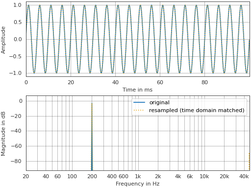
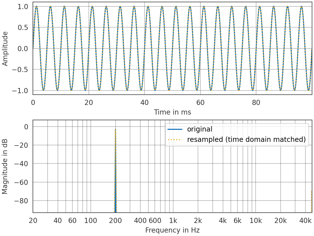
For power signals, the amplitude of the resampled signal is automatically correct in the time and frequency domain if
match_amplitude="time">>> import pyfar as pf >>> import matplotlib.pyplot as plt >>> >>> signal = pf.signals.sine(200, 4800, sampling_rate=48000) >>> resampled = pf.dsp.resample(signal, 96000) >>> >>> pf.plot.time_freq(signal, label="original", unit='ms') >>> pf.plot.time_freq(resampled, c="y", ls=":", unit='ms', ... label="resampled (time domain matched)") >>> plt.legend()
(
Source code,png,hires.png,pdf)
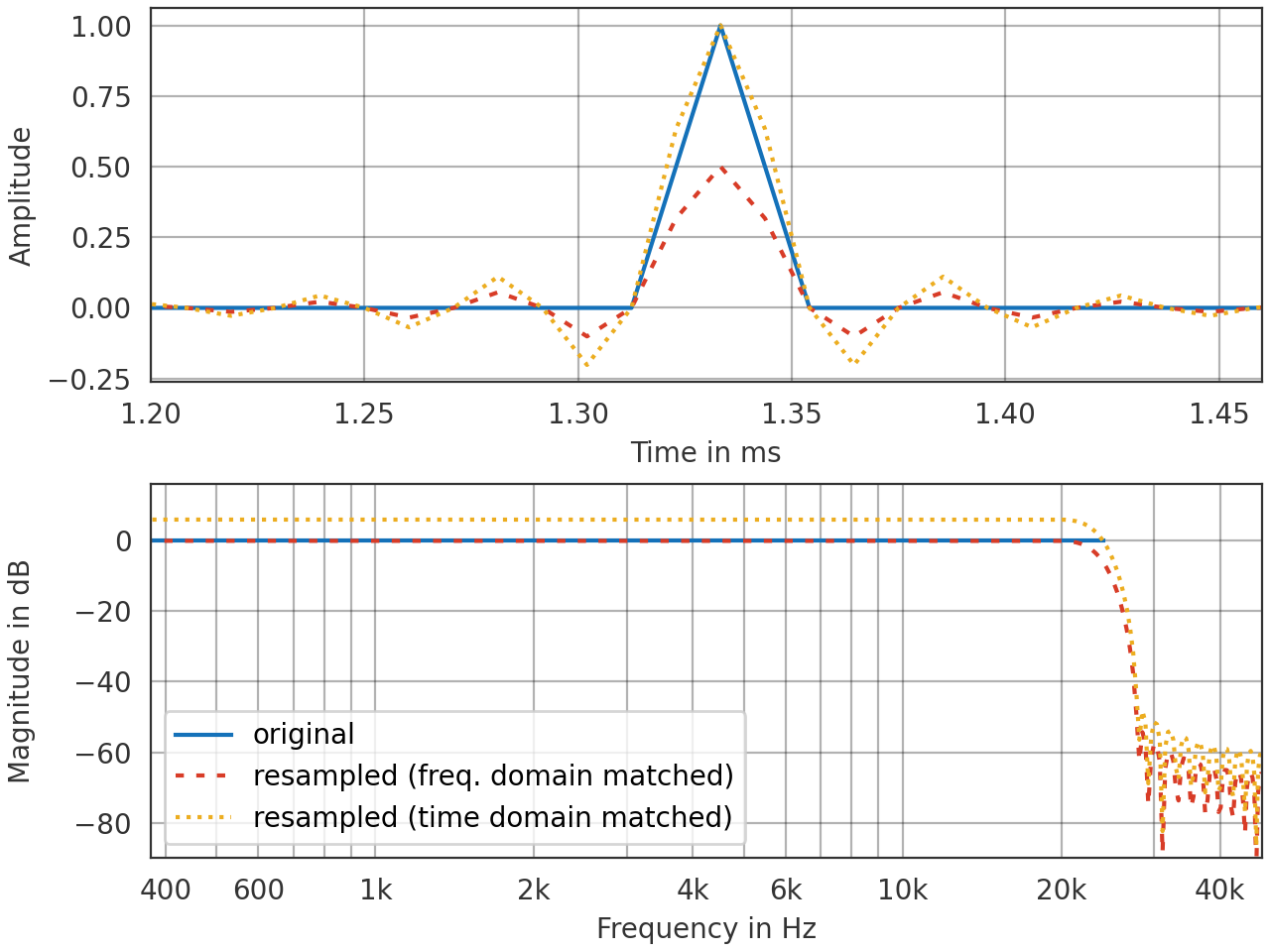
With some energy signals, such as impulse responses, the amplitude can only be correct in the time or frequency domain due to the lack of normalization by the number of samples. In such cases, it is often desired to match the amplitude in the frequency domain
>>> import pyfar as pf
>>> import matplotlib.pyplot as plt
>>>
>>> signal = pf.signals.impulse(128, 64, sampling_rate=48000)
>>> resampled_time = pf.dsp.resample(
...     signal, 96000, match_amplitude = "time")
>>> resampled_freq = pf.dsp.resample(
...     signal, 96000, match_amplitude = "freq")
>>>
>>> pf.plot.time_freq(signal, label="original", unit='ms')
>>> pf.plot.time_freq(resampled_freq, dashes=[2, 3], unit='ms',
...                   label="resampled (freq. domain matched)")
>>> ax = pf.plot.time_freq(resampled_time, ls=":", unit='ms',
...                   label="resampled (time domain matched)", c='y')
>>> ax[0].set_xlim(1.2,1.46)
>>> plt.legend()
(
Source code,png,hires.png,pdf)
- pyfar.dsp.rms(signal)[source]#
Compute the root mean square (RMS) of a signal.
The RMS is calculated as
\[\sqrt{\frac{1}{N}\sum_{n=0}^{N-1}|x[n]|^2}\]based on the time data for each channel separately.
- Parameters:
signal (Signal) – The signal to compute the RMS from.
- Returns:
data – The channel-wise RMS of the input signal.
- Return type:
Notes
The RMS equals the square root of the signal’s power.
energyandpowercan be used to compute the energy and the power.
- pyfar.dsp.smooth_fractional_octave(signal, num_fractions, mode='magnitude_zerophase', window='boxcar')[source]#
Smooth spectrum with a fractional octave width.
The smoothing is done according to Tylka et al. 2017 [13] (method 2) in three steps:
Interpolate the spectrum to a logarithmically spaced frequency scale
Smooth the spectrum by convolution with a smoothing window
Interpolate the spectrum to the original linear frequency scale
Smoothing of complex-valued time data is not implemented.
- Parameters:
signal (pyfar.Signal) – The input data.
num_fractions (number) – The width of the smoothing window in fractional octaves, e.g., 3 will apply third octave smoothing and 1 will apply octave smoothing.
mode (str, optional) –
"magnitude_zerophase"Only the magnitude response, i.e., the absolute spectrum is smoothed. Note that this return a zero-phase signal. It might be necessary to generate a minimum or linear phase if the data is subject to further processing after the smoothing (cf.
minimum_phaseandlinear_phase)"magnitude"Smooth the magnitude and keep the phase of the input signal.
"magnitude_phase"Separately smooth the magnitude and unwrapped phase response.
"complex"Separately smooth the real and imaginary part of the spectrum.
Note that the modes magnitude_zerophase and magnitude make sure that the smoothed magnitude response is as expected at the cost of an artificial phase response. This is often desired, e.g., when plotting signals or designing compensation filters. The modes magnitude_phase and complex smooth all information but might cause a high frequency energy loss in the smoothed magnitude response. The default is
"magnitude_zerophase".window (str, optional) – String that defines the smoothing window. All windows from
time_windowthat do not require an additional parameter can be used. The default is “boxcar”, which uses the most commonly used rectangular window.
- Returns:
signal (pyfar.Signal) – The smoothed output data
window_stats (tuple) – A tuple containing information about the smoothing process
- n_window
The window length in (logarithmically spaced) samples
- num_fractions
The actual width of the window in fractional octaves. This can deviate from the desired width because the smoothing window must have an integer sample length
Notes
Method 3 in Tylka at al. 2017 is mathematically more elegant at the price of a largely increased computational and memory cost. In most practical cases, methods 2 and 3 yield close to identical results (cf. Fig. 2 and 3 in Tylka et al. 2017). If the spectrum contains extreme discontinuities, however, method 3 is superior (see examples below).
References
Examples
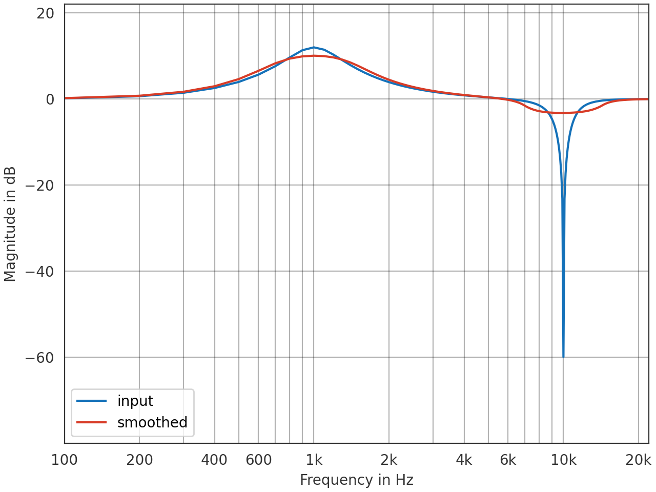
Octave smoothing of continuous spectrum consisting of two bell filters.
>>> import pyfar as pf
>>> signal = pf.signals.impulse(441)
>>> signal = pf.dsp.filter.bell(signal, 1e3, 12, 1, "III")
>>> signal = pf.dsp.filter.bell(signal, 10e3, -60, 100, "III")
>>> smoothed, _ = pf.dsp.smooth_fractional_octave(signal, 1)
>>> ax = pf.plot.freq(signal, label="input")
>>> pf.plot.freq(smoothed, label="smoothed")
>>> ax.legend(loc=3)
(
Source code,png,hires.png,pdf)
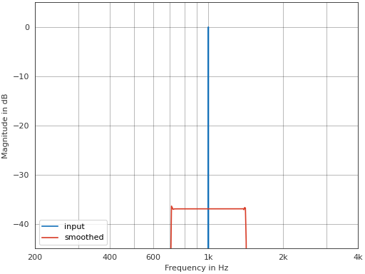
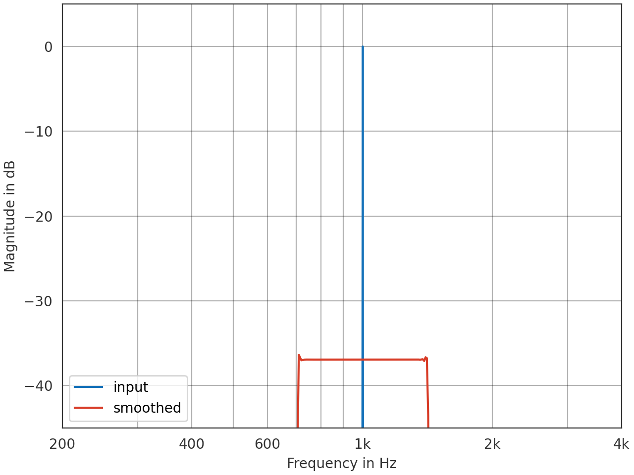
Octave smoothing of the discontinuous spectrum of a sine signal causes artifacts at the edges due to the intermediate interpolation steps (cf. Tylka et al. 2017, Fig. 4). However this is a rather unusual application and is mentioned only for the sake of completeness.
>>> import pyfar as pf
>>> signal = pf.signals.sine(1e3, 4410)
>>> signal.fft_norm = "amplitude"
>>> smoothed, _ = pf.dsp.smooth_fractional_octave(signal, 1)
>>> ax = pf.plot.freq(signal, label="input")
>>> pf.plot.freq(smoothed, label="smoothed")
>>> ax.set_xlim(200, 4e3)
>>> ax.set_ylim(-45, 5)
>>> ax.legend(loc=3)
(
Source code,png,hires.png,pdf)
- pyfar.dsp.soft_limit_spectrum(signal, limit, knee, frequency_range=None, direction='upper', log_prefix=None)[source]#
Soft limiting the magniude spectrum.
Soft limiting gradually increases the gain reduction to avoid discontinuities in the data that would appear in hard limiting. The transition between the magnitude where no limiting is applied to the magnitude where the limiting reaches its full effect is termed knee (see examples below).
Note that the limiting is applied on signal.freq, i.e. the data after the FFT normalization.
- Parameters:
signal (Signal, FrequencyData) – The input data
limit (number, array like) – The gain in dB at which the limiting reaches its full effect. If this is a number, the same limit is applied to all frequencies. If this an array like, it must be broadcastable to
signal.freqto apply frequency-dependent limits.knee (number, string) – If this is a number, a knee with a width of number dB according to [14] Eq. (4) is applied. This definition of the knee originates from the classic limiting audio effect. If this is
'arctan'an arcus tangens knee according to [15] Section 3.6.4 is applied. This knee definition originates from microphone array signal processing.frequency_range (array like, optional) – Frequency range in which the limiting is applied. This must be an array like containing the lower and upper limit in Hz. The default
Noneapplies the limiting to all frequencies.direction (str, optional) –
Define how the limiting works
'upper'(default)Soft limiting signal to enforce an aboslute maximum value of limit.
'lower'Soft limiting signal to enforce an absolute minimum value of limit
log_prefix (float, int) – The log prefix is used to linearize the limit and knee, e.g.,
limit_linear = 10**(limit / log_prefix).The defaultNone, uses10for signals with'psd'and'power'FFT normalization and20otherwise.
- Returns:
limited – The limited copy of the input data.
- Return type:
Examples
Illustrate effect of limit and knee
>>> import pyfar as pf
>>> import numpy as np
>>>
>>> signal = pf.FrequencyData(
...     10**(np.arange(-20, 21)/20), np.arange(0, 41))
>>> for knee in ['arctan', 20, 0]:
>>>     limited = pf.dsp.soft_limit_spectrum(signal, 0, knee)
>>>     pf.plot.freq(limited, freq_scale='linear', label=f'{knee=}')
>>> ax = pf.plot.freq(signal, freq_scale='linear',
...                   linestyle='--', label='input')
>>>
>>> ax.legend(loc='upper left')
>>> ax.set_xlim(0, 40)
>>> ax.set_ylim(-20, 20)
>>> bbox=dict(facecolor='white', edgecolor='none', alpha=0.5)
>>> arrowprops= dict(
...     arrowstyle="<->", shrinkA=0, shrinkB=0,
...     color=pf.plot.color('r'))
>>> ax.annotate("limit=0 dB", (20, 0), (10, 0), bbox=bbox,
...             arrowprops=dict(arrowstyle="->"), va='center')
>>> ax.text(20, -14, 'knee=20 dB', ha='center',
...         color=pf.plot.color('r'), bbox=bbox)
>>> ax.annotate("", (10, -15), (30, -15), arrowprops=arrowprops)
(
Source code,png,hires.png,pdf)
Apply limiting with knee (soft limiting) and without knee (hard limiting)
>>> import pyfar as pf
>>>
>>> signal = pf.signals.impulse(4096)
>>> signal = pf.dsp.filter.bell(signal, 1e3, 20, 1)
>>>
>>> soft = pf.dsp.soft_limit_spectrum(signal, limit=10, knee=12)
>>> hard = pf.dsp.soft_limit_spectrum(signal, limit=10, knee=0)
>>>
>>> pf.plot.freq(soft, label='soft (knee > 0)')
>>> pf.plot.freq(hard, label='hard (knee = 0)')
>>> ax = pf.plot.freq(signal, ls='--', label='original')
>>>
>>> ax.set_ylim(-5, 25)
>>> ax.legend()
(
Source code,png,hires.png,pdf)
Apply soft limiting above and below +/-10 dB
>>> import pyfar as pf
>>>
>>> signal = pf.signals.impulse(4096)
>>> signal = pf.dsp.filter.bell(signal, 2e2, -20, 3)
>>> signal = pf.dsp.filter.bell(signal, 6e3, 20, 3)
>>>
>>> upper = pf.dsp.soft_limit_spectrum(
...     signal, limit=10, knee=6, direction="upper")
>>> lower = pf.dsp.soft_limit_spectrum(
...     signal, limit=-10, knee=6, direction="lower")
>>>
>>> pf.plot.freq(upper, label='upper limit')
>>> pf.plot.freq(lower, label='lower limit')
>>> ax = pf.plot.freq(signal, ls='--', label='original')
>>>
>>> ax.set_ylim(-25, 25)
>>> ax.legend()
(
Source code,png,hires.png,pdf)
Apply frequency dependent soft limiting
>>> import pyfar as pf
>>>
>>> # input data
>>> signal = pf.signals.impulse(2**13)
>>> signal = pf.dsp.filter.bell(signal, 2e2, 20, 4)
>>> signal = pf.dsp.filter.bell(signal, 2e3, 20, 4)
>>>
>>> # frequency dependent limit
>>> limit = pf.dsp.filter.low_shelf(
...     pf.signals.impulse(2**13), 500, -10, 2) * 10
>>> limit = pf.dsp.decibel(limit).flatten()
>>>
>>> # soft limiting input signal
>>> limited = pf.dsp.soft_limit_spectrum(signal, limit, 10)
>>>
>>> # plot
>>> ax = pf.plot.freq(signal, label='original')
>>> pf.plot.freq(limited, label='limited')
>>> ax.plot(signal.frequencies, limit, label='limit', c='k', ls='--')
>>> ax.set_ylim(-5, 25)
>>> ax.legend(loc='upper left')
(
Source code,png,hires.png,pdf)
References
- pyfar.dsp.spectrogram(signal, window='hann', window_length=1024, window_overlap_fct=0.5, normalize=True)[source]#
Compute the magnitude spectrum versus time.
This is a wrapper for
scipy.signal.ShortTimeFFT.spectrogramwith two differences. First, the returned times refer to the start of the FFT blocks, i.e., the first time is always 0 whereas it is window_length/2 in scipy. Second, the returned spectrogram is normalized according tosignal.fft_normif thenormalizeparameter is set toTrue.- Parameters:
signal (Signal) – Signal to compute spectrogram of.
window (str) – Specifies the window (see
scipy.signal.windows). The default is'hann'.window_length (integer) – Window length in samples, the default ist 1024.
window_overlap_fct (double) – Ratio of points to overlap between FFT segments [0…1]. The default is
0.5.normalize (bool) – Flag to indicate if the FFT normalization should be applied to the spectrogram according to signal.fft_norm. The default is
True.
- Returns:
frequencies (numpy array) – Frequencies in Hz at which the magnitude spectrum was computed. For complex valued signals, frequencies and spectrogram is arranged such that 0 Hz bin is centered.
times (numpy array) – Times in seconds at which the magnitude spectrum was computed
spectrogram (numpy array)
- pyfar.dsp.time_crop(signal, interval: list[float] | tuple[float, float] | ndarray, unit: Literal['samples', 's'] = 'samples')[source]#
Crop a
Signalor aTimeDataobject in time.Returns the signal \(x(t)\) defined for all \(t\) within the interval \(interval[0] \le t \le interval[1]\), where \(t\) can be time or samples.
- Parameters:
signal (pyfar.Signal, pyfar.TimeData) –
SignalorTimeDataobject to be cropped.interval (list, tuple, or numpy.ndarray) – Must contain exactly two entries, these specify the beginning and the end of the section to be cropped. The unit of interval is specified by the parameter unit.
unit (string, optional) – Unit of interval. Can be set to
'samples'or's'(seconds). Values in seconds are rounded to the nearest sample within the specified interval range. The default is'samples'.
- Returns:
- Return type:
Notes
For
Signal, the starting point of the cropped signal is always set to zero, while forTimeData, the starting point is set to the point where cropping begins in the original signal.Examples
Create a sine wave signal and extract an interval from it. The starting point of the cropped signal is reset to zero.
>>> import pyfar as pf
>>> import numpy as np
>>> import matplotlib.pyplot as plt
>>> fig, (ax1, ax2) = plt.subplots(2, 1)
>>> plt.subplots_adjust(hspace=0.33)
>>> signal = pf.signals.sine(100, 4410)
>>> signal_cropped = pf.dsp.time_crop(signal, interval=[565, 1220])
>>> pf.plot.time(signal, label='original',
...                             unit = 'samples', ax=ax1)
>>> ax1.axvline(565, color='k', linestyle='-.', label='interval')
>>> ax1.axvline(1220, color='k',  linestyle='-.')
>>> pf.plot.time(signal_cropped, color='y',
...     label='cropped', unit='samples', ax=ax2)
>>> for ax in [ax1, ax2]:
>>>     ax.legend()
>>> fig.suptitle('Crop a Signal object')
(
Source code,png,hires.png,pdf)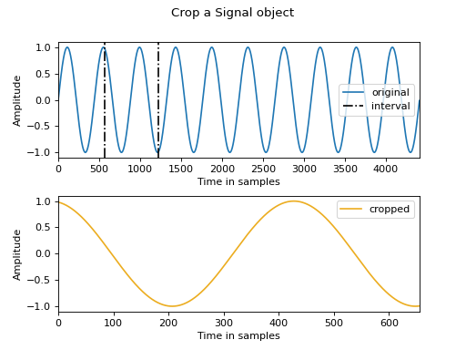
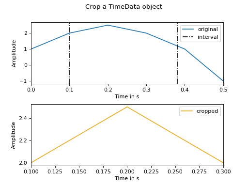
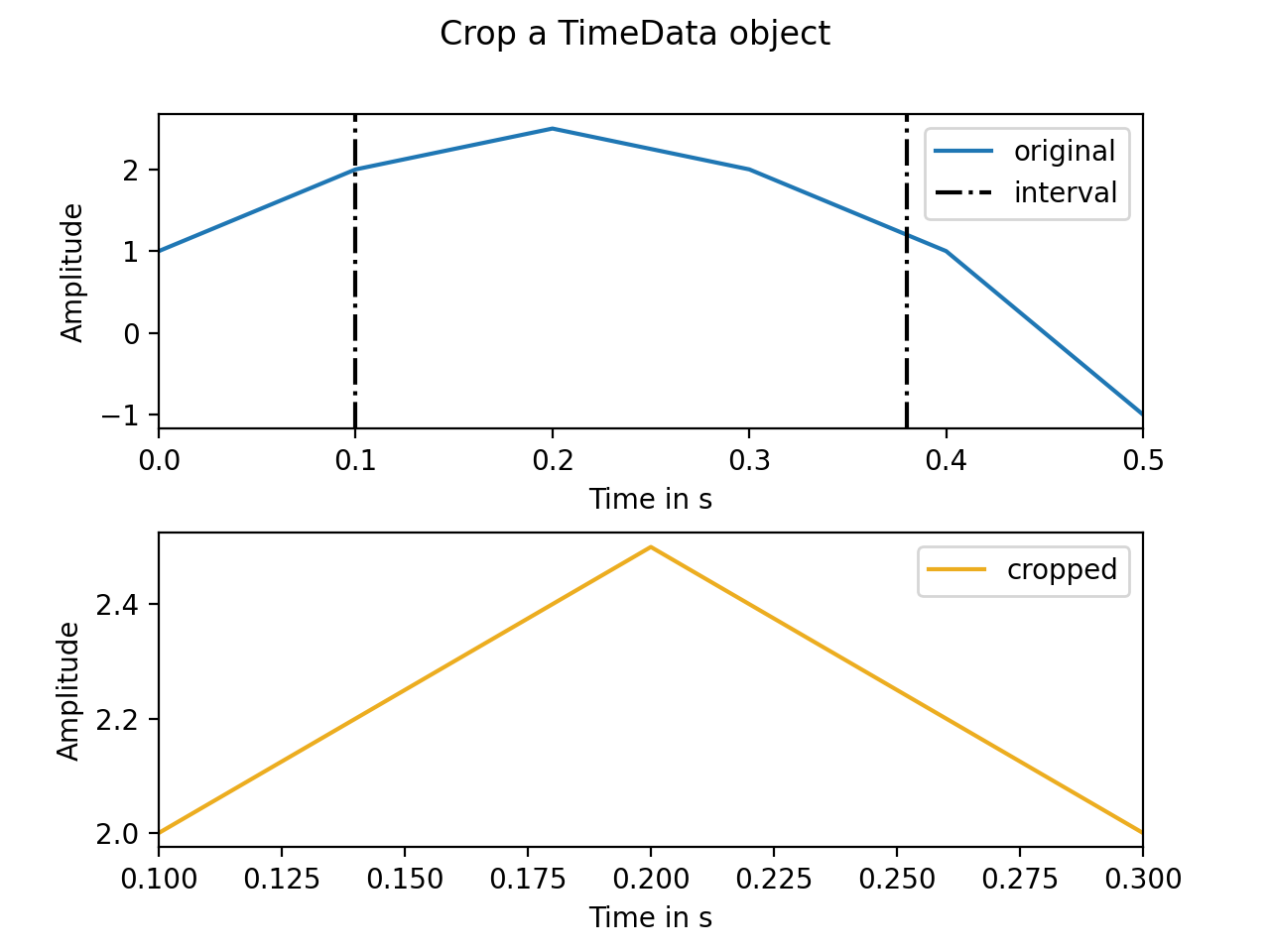
Create a TimeData object and extract an interval from it. The starting point in time is NOT reset; the cropped signal starts from the time instance closest to the first point in the interval.
>>> import pyfar as pf
>>> import numpy as np
>>> import matplotlib.pyplot as plt
>>> fig, (ax3, ax4) = plt.subplots(2, 1)
>>> plt.subplots_adjust(hspace=0.33)
>>> time_signal = pf.TimeData((1, 2, 2.5, 2, 1, -1 ),
...                             (0, 0.1, 0.2, 0.3, 0.4, 0.5))
>>> time_signal_cropped = pf.dsp.time_crop(time_signal,
...                             interval=[0.1, 0.38], unit='s')
>>> pf.plot.time(time_signal, label='original',
...                                             unit = 's', ax=ax3)
>>> ax3.axvline(0.1, color='k', linestyle='-.', label='interval')
>>> ax3.axvline(0.38, color='k',  linestyle='-.')
>>> pf.plot.time(time_signal_cropped, color='y',
...     label='cropped', unit = 's', ax=ax4)
>>> for ax in [ax3, ax4]:
>>>     ax.legend()
>>> fig.suptitle('Crop a TimeData object')
(
Source code,png,hires.png,pdf)
- pyfar.dsp.time_shift(signal, shift, mode='cyclic', unit='samples', pad_value=0.0)[source]#
Apply a cyclic or linear time-shift to a signal.
This function only allows integer value sample shifts. If unit
'time'is used, the shift samples will be rounded to the nearest integer value. For a shift using fractional sample values seefractional_time_shift.- Parameters:
signal (Signal) – The signal to be shifted
shift (int, float, array_like) – The time-shift value. A positive value will result in right shift on the time axis (delaying of the signal), whereas a negative value yields a left shift on the time axis (non-causal shift to a earlier time). If a single value is given, the same time shift will be applied to each channel of the signal. Individual time shifts for each channel can be performed by passing an array broadcastable to the signals channel dimensions
cshape.mode (str, optional) –
The shifting mode
"linear"Apply linear shift, i.e., parts of the signal that are shifted to times smaller than 0 samples and larger than
signal.n_samplesdisappear. To maintain the shape of the signal, the signal is padded at the respective other end. The pad value is determined bypad_type."cyclic"Apply a cyclic shift, i.e., parts of the signal that are shifted to values smaller than 0 are wrapped around to the end, and parts that are shifted to values larger than
signal.n_samplesare wrapped around to the beginning.
The default is
"cyclic"unit (str, optional) – Unit of the shift variable, this can be either
'samples'or's'for seconds. By default'samples'is used. Note that in the case of specifying the shift time in seconds, the value is rounded to the next integer sample value to perform the shift.pad_value (numeric, optional) – The pad value for linear shifts, by default
0.is used. Padnumpy.nanto the respective channels if the rms value of the signal is to be maintained for block-wise rms estimation of the noise power of a signal. Note that if NaNs are padded, the returned data will be aTimeDatainstead ofSignalobject.
- Returns:
The time-shifted signal. This is a
TimeDataobject in case a linear shift was done and the signal was padded with Nans. In all other cases, aSignalobject is returned.- Return type:
Examples
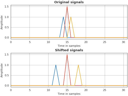
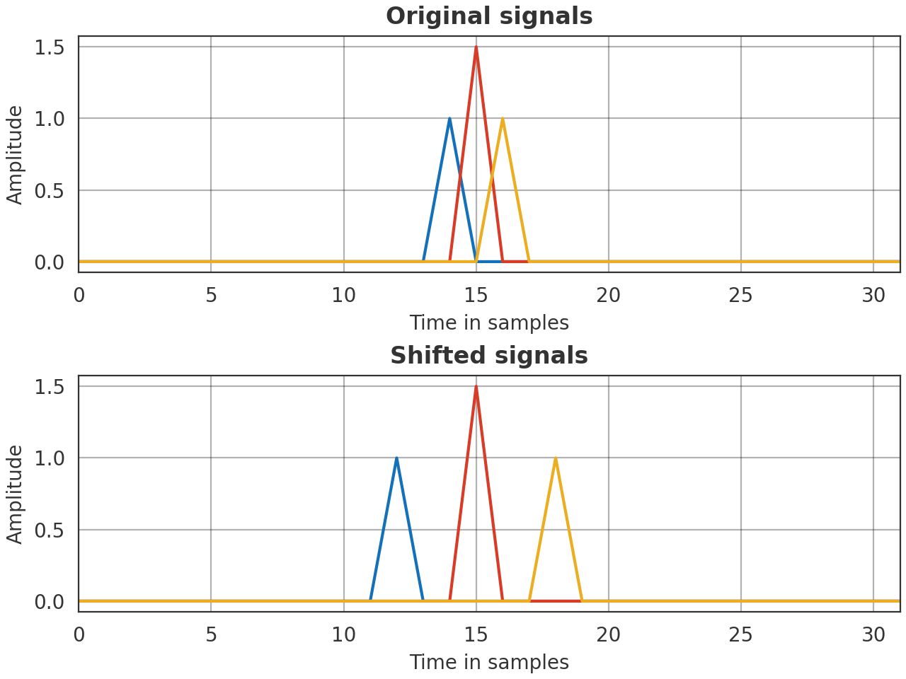
Individually do a cyclic shift of a set of ideal impulses stored in three different channels and plot the resulting signals
>>> import pyfar as pf
>>> import matplotlib.pyplot as plt
>>> # generate and shift the impulses
>>> impulse = pf.signals.impulse(
...     32, amplitude=(1, 1.5, 1), delay=(14, 15, 16))
>>> shifted = pf.dsp.time_shift(impulse, [-2, 0, 2])
>>> # time domain plot
>>> pf.plot.use('light')
>>> _, axs = plt.subplots(2, 1)
>>> pf.plot.time(impulse, ax=axs[0], unit='samples')
>>> pf.plot.time(shifted, ax=axs[1], unit='samples')
>>> axs[0].set_title('Original signals')
>>> axs[1].set_title('Shifted signals')
(
Source code,png,hires.png,pdf)
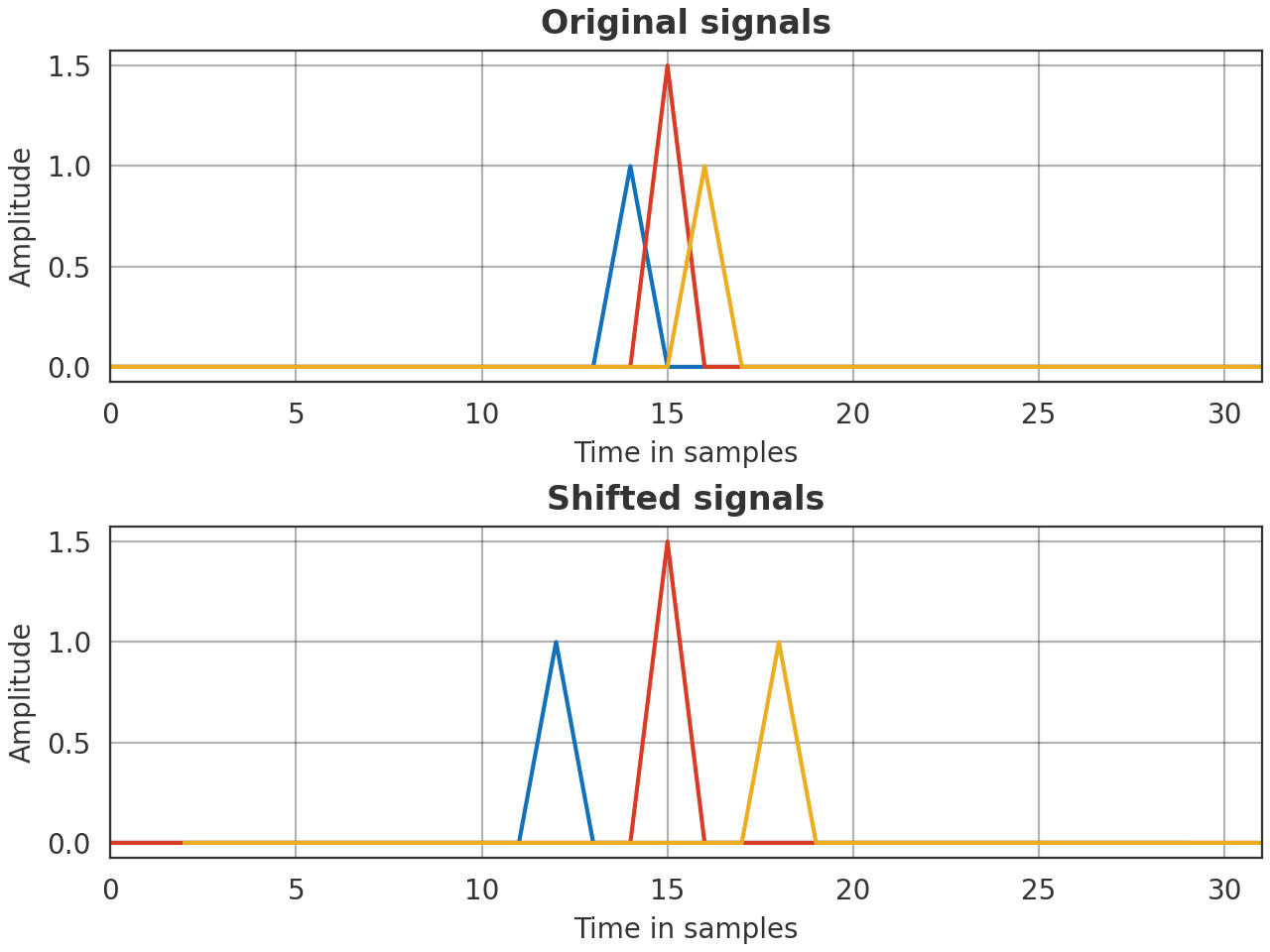
Perform a linear time shift instead and pad with NaNs
>>> import pyfar as pf
>>> import numpy as np
>>> import matplotlib.pyplot as plt
>>> # generate and shift the impulses
>>> impulse = pf.signals.impulse(
...     32, amplitude=(1, 1.5, 1), delay=(14, 15, 16))
>>> shifted = pf.dsp.time_shift(
...     impulse, [-2, 0, 2], mode='linear', pad_value=np.nan)
>>> # time domain plot
>>> pf.plot.use('light')
>>> _, axs = plt.subplots(2, 1)
>>> pf.plot.time(impulse, ax=axs[0], unit='samples')
>>> pf.plot.time(shifted, ax=axs[1], unit='samples')
>>> axs[0].set_title('Original signals')
>>> axs[1].set_title('Shifted signals')
(
Source code,png,hires.png,pdf)
- pyfar.dsp.time_window(signal, interval, window='hann', shape='symmetric', unit='samples', crop='none', return_window=False)[source]#
Apply time window to signal.
This function uses the windows implemented in
scipy.signal.windows.- Parameters:
signal (Signal) – Signal object to be windowed.
interval (array_like) – If interval has two entries, these specify the beginning and the end of the symmetric window or the fade-in / fade-out (see parameter shape). If interval has four entries, a window with fade-in between the first two entries and a fade-out between the last two is created, while it is constant in between (ignores shape). The unit of interval is specified by the parameter unit. See below for more details.
window (string, float, or tuple, optional) – The type of the window. See below for a list of implemented windows. The default is
'hann'.shape (string, optional) –
'symmetric'General symmetric window, the two values in interval define the first and last samples of the window.
'symmetric_zero'Symmetric window with respect to t=0, the two values in interval define the first and last samples of fade-out. crop is ignored.
'left'Fade-in, the beginning and the end of the fade is defined by the two values in interval. See Notes for more details.
'right'Fade-out, the beginning and the end of the fade is defined by the two values in interval. See Notes for more details.
The default is
'symmetric'.unit (string, optional) – Unit of interval. Can be set to
'samples'or's'(seconds). Time values are rounded to the nearest sample. The default is'samples'.crop (string, optional) –
'none'The length of the windowed signal stays the same.
'window'The signal is truncated to the windowed part.
'end'Only the zeros at the end of the windowed signal are cropped, so the original phase is preserved.
The default is
'none'.return_window (bool, optional) – If
True, both the windowed signal and the time window are returned. The default isFalse.
- Returns:
signal_windowed (Signal) – Windowed signal object
window (Signal) – Time window used to create the windowed signal, only returned if
return_window=True.
Notes
For a fade-in, the indexes of the samples given in interval denote the first sample of the window which is non-zero and the first which is one. For a fade-out, the samples given in interval denote the last sample which is one and the last which is non-zero.
This function calls
scipy.signal.windows.get_windowto create the window. Available window types:boxcartriangblackmanhamminghannbartlettflattopparzenbohmanblackmanharrisnuttallbarthannkaiser(needs beta, seekaiser_window_beta)gaussian(needs standard deviation)general_gaussian(needs power, width)dpss(needs normalized half-bandwidth)chebwin(needs attenuation)exponential(needs center, decay scale)tukey(needs taper fraction)taylor(needs number of constant sidelobes, sidelobe level)
If the window requires no parameters, then window can be a string. If the window requires parameters, then window must be a tuple with the first argument the string name of the window, and the next arguments the needed parameters.
Examples
Options for parameter shape.
>>> import pyfar as pf
>>> import numpy as np
>>> signal = pf.Signal(np.ones(100), 44100)
>>> for shape in ['symmetric', 'symmetric_zero', 'left', 'right']:
>>>     signal_windowed = pf.dsp.time_window(
...         signal, interval=[25,45], shape=shape)
>>>     ax = pf.plot.time(signal_windowed, label=shape, unit='ms')
>>> ax.legend(loc='right')
(
Source code,png,hires.png,pdf)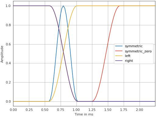
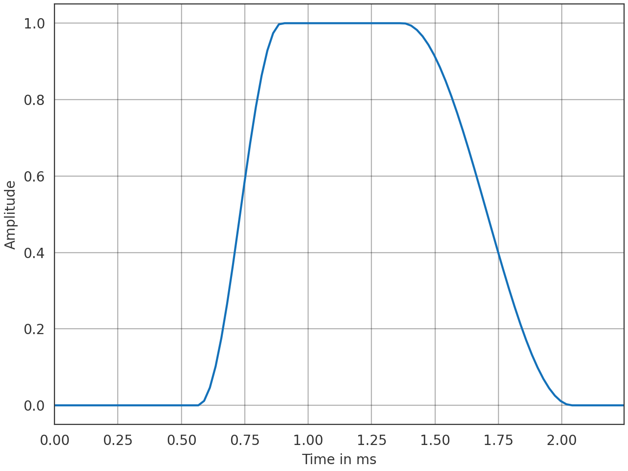
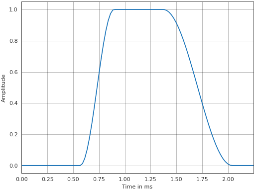
Window with fade-in and fade-out defined by four values in interval.
>>> import pyfar as pf
>>> import numpy as np
>>> signal = pf.Signal(np.ones(100), 44100)
>>> signal_windowed = pf.dsp.time_window(
...         signal, interval=[25, 40, 60, 90], window='hann')
>>> pf.plot.time(signal_windowed, unit='ms')
(
Source code,png,hires.png,pdf)
- pyfar.dsp.wrap_to_2pi(x)[source]#
Wraps phase to 2 pi.
- Parameters:
x (double) – Input phase to be wrapped to 2 pi.
- Returns:
x – Phase wrapped to 2 pi`.
- Return type:
double
- pyfar.dsp.zero_phase(signal)[source]#
Calculate zero phase signal.
The zero phase signal is obtained by taking the absolute values of the spectrum
\[H_z = |H| = \sqrt{\mathrm{real}(H)^2 + \mathrm{imag}(H)^2},\]where \(H\) is the complex valued spectrum of the input data and \(H_z\) the real valued zero phase spectrum.
The time domain data of a zero phase signal is symmetric around the first sample, e.g.,
signal.time[0, 1] == signal.time[0, -1].- Parameters:
signal (Signal, FrequencyData) – input data
- Returns:
signal – zero phase copy of the input data
- Return type: