pyfar.constants

Module for constants and physical properties of air.

Constants:

pyfar.constants.absolute_zero_celsius: Final[float] = -273.15

Absolute zero temperature \(\mathrm{t_0}\) in degree Celsius [1].

\[t_0 = -273.15 \text{°C}\]

Returns:

t_0 – Absolute zero temperature in degree Celsius.

Return type:

float

References

[1]

https://en.wikipedia.org/wiki/Absolute_zero

pyfar.constants.reference_air_density: Final[float] = 1.204

Reference air density in \(\text{kg}/\text{m}^3\) at reference atmospheric pressure and 20°C [2].

\[\rho_\text{atm} = 1.204 \, \frac{\text{kg}}{\text{m}^3}\]

Returns:

Reference air density in \(\text{kg}/\text{m}^3\).

Return type:

float

References

[2]

https://en.wikipedia.org/wiki/Density_of_air

pyfar.constants.reference_air_impedance: Final[float] = 413.21279999999996

Reference air impedance \(Z_\text{ref}\) in Pa s/m is calculated based on reference_speed_of_sound and standard_air_density.

\[Z_\text{ref} = \rho_\text{atm} \cdot c_\text{ref} \approx 413.2 \, \text{Pa s/m}\]

Returns:

Z_ref – Reference air impedance in Pa s/m.

Return type:

float

pyfar.constants.reference_air_temperature_celsius: Final[float] = 20

Reference air temperature \(t_\text{ref}\) in degree Celsius [3].

\[t_\text{ref} = 20 \text{°C}\]

Returns:

t_ref – Reference air temperature in degree Celsius.

Return type:

float

References

[3]

ISO 9613-1:1993, Acoustics – Attenuation of sound during propagation outdoors – Part 1: Calculation of the absorption of sound by the atmosphere.

pyfar.constants.reference_atmospheric_pressure: Final[float] = 101325.0

Reference atmospheric pressure \(P_\text{atm}\) in Pascal [4].

\[P_\text{atm} = 101325 \, \text{Pa}\]

Returns:

Reference atmospheric pressure in Pascal.

Return type:

float

References

[4]

https://en.wikipedia.org/wiki/Atmospheric_pressure

pyfar.constants.reference_sound_power: Final[float] = 1e-12

Reference sound power \(P_\text{ref}\) in Watt [5].

\[P_\text{ref} = 1 \, \text{pW} = 10^{-12} \, \text{W}\]

Returns:

P_ref – Reference sound power in Watt.

Return type:

float

References

[5]

https://asastandards.org/terms/sound-power-level/

pyfar.constants.reference_sound_pressure: Final[float] = 2e-05

Reference sound pressure \(p_\text{ref}\) in Pascal [6].

\[p_\text{ref} = 20 \, \mathrm{\mu Pa}\]

Returns:

p_ref – Reference sound pressure in Pascal.

Return type:

float

References

[6]

https://asastandards.org/terms/reference-value-for-sound-pressure-2/

pyfar.constants.reference_speed_of_sound: Final[float] = 343.2

Reference speed of sound \(c_\text{ref}\) in m/s for 20°C and dry air [7].

\[c_\text{ref} = 343.2 \, \text{m/s}\]

Returns:

c_ref – Reference speed of sound in m/s.

Return type:

float

References

[7]

ISO 9613-1:1993, Acoustics – Attenuation of sound during propagation outdoors – Part 1: Calculation of the absorption of sound by the atmosphere.

Functions:

air_attenuation(temperature, frequencies, ...)	Calculate the pure tone attenuation of sound in air according to ISO 9613-1.
density_of_air(temperature, relative_humidity)	Calculate the density of air in kg/m³ based on the temperature, relative humidity, and atmospheric pressure.
fractional_octave_filter_tolerance(...)	Calculate the tolerance limits for fractional octave band filters.
fractional_octave_frequencies_exact([...])	Return the exact center and cutoff frequencies for fractional-octave-band filters.
fractional_octave_frequencies_nominal([...])	Return the nominal center frequencies for octave-band and one-third-octave-band filters.
frequency_weighting_band_corrections(...)	Returns the A or C frequency weighting correction values for octave or third-octave bands in a given frequency range.
frequency_weighting_curve(weighting, frequencies)	Calculates the level correction in dB of each frequency component when using the A or C frequency weighting.
saturation_vapor_pressure_magnus(temperature)	Calculate the saturation vapor pressure of water in Pascal using the Magnus formula.
speed_of_sound_cramer(temperature, ...[, ...])	Calculate the speed of sound in air based on temperature, atmospheric pressure, humidity and CO2 concentration.
speed_of_sound_ideal_gas(temperature, ...[, ...])	Calculate speed of sound in air using the ideal gas law.
speed_of_sound_simple(temperature)	Calculate the speed of sound in air using a simplified version of the ideal gas law based on the temperature.

pyfar.constants.air_attenuation(temperature, frequencies, relative_humidity, atmospheric_pressure=None)

Calculate the pure tone attenuation of sound in air according to ISO 9613-1.

Calculation is in accordance with ISO 9613-1 [8]. The shape of the outputs is broadcasted from the shapes of the temperature, relative_humidity, and atmospheric_pressure. The frequency bins represents the last dimension.

Parameters:

• temperature (float, array_like) – Temperature in °C. Must be in the range of -20 °C to 50 °C for accuracy of +/-10% or must be greater than -70 °C for accuracy of +/-50%.

• frequencies (float, array_like) – Frequency in Hz. Must be greater than 50 Hz. Just one dimensional array is allowed.

• relative_humidity (float, array_like) – Relative humidity in the range from 0 to 1.

• atmospheric_pressure (float, array_like, optional) – Atmospheric pressure in Pascal, by default reference_atmospheric_pressure.

Returns:

• alpha (np.ndarray[float]) – Pure tone air attenuation coefficient in dB/m for atmospheric absorption.

• m (FrequencyData) – Pure tone energy attenuation coefficient in 1/m for atmospheric absorption. The parameter m is calculated as \(m = \alpha / (10 \log_{10}(e))\).

• accuracy (FrequencyData) – accuracy of the results according to the standard:

  10, +/- 10% accuracy

  • molar concentration of water vapour: 0.05% to 5%.

  • air temperature: 253.15 K to 323.15 K (-20 °C to +50 °C)

  • atmospheric pressure: less than 200 000 Pa (2 atm)

  • frequency-to-pressure ratio: 0.0004 Hz/Pa to 10 Hz/Pa.

  20, +/- 20% accuracy

  • molar concentration of water vapour: 0.005% to 0.05%, and greater than 5%

  • air temperature: 253.15 K to 323.15 K (-20 °C to +50 °C)

  • atmospheric pressure: less than 200 000 Pa (2 atm)

  • frequency-to-pressure ratio: 0.0004 Hz/Pa to 10 Hz/Pa.

  50, +/- 50% accuracy

  • molar concentration of water vapour: less than 0.005%

  • air temperature: greater than 200 K (- 73 °C)

  • atmospheric pressure: less than 200 000 Pa (2 atm)

  • frequency-to-pressure ratio: 0.0004 Hz/Pa to 10 Hz/Pa.

  -1, no valid result

  else.

References

[8]

ISO 9613-1:1993, Acoustics – Attenuation of sound during propagation outdoors – Part 1: Calculation of the absorption of sound by the atmosphere.

pyfar.constants.density_of_air(temperature, relative_humidity, atmospheric_pressure=None, saturation_vapor_pressure=None)

Calculate the density of air in kg/m³ based on the temperature, relative humidity, and atmospheric pressure.

The density of air is calculated based on chapter 6.3 in [9]. All input parameters must be broadcastable to the same shape.

Parameters:

• temperature (float, array_like) – Temperature in degrees Celsius (°C).

• relative_humidity (float, array_like) – Relative humidity in the range from 0 to 1.

• atmospheric_pressure (float, array_like, optional) – Atmospheric pressure in Pascal (Pa), by default reference_atmospheric_pressure.

• saturation_vapor_pressure (float, array_like, optional) – Saturation vapor pressure in Pascal (Pa). The default uses the value and valid temperature range from saturation_vapor_pressure_magnus.

Returns:

density – Density of air in kg/m³.

Return type:

float, array_like

References

[9]

V. E. Ostashev and D. K. Wilson, Acoustics in Moving Inhomogeneous Media, 2nd ed. London: CRC Press, 2015. doi: 10.1201/b18922.

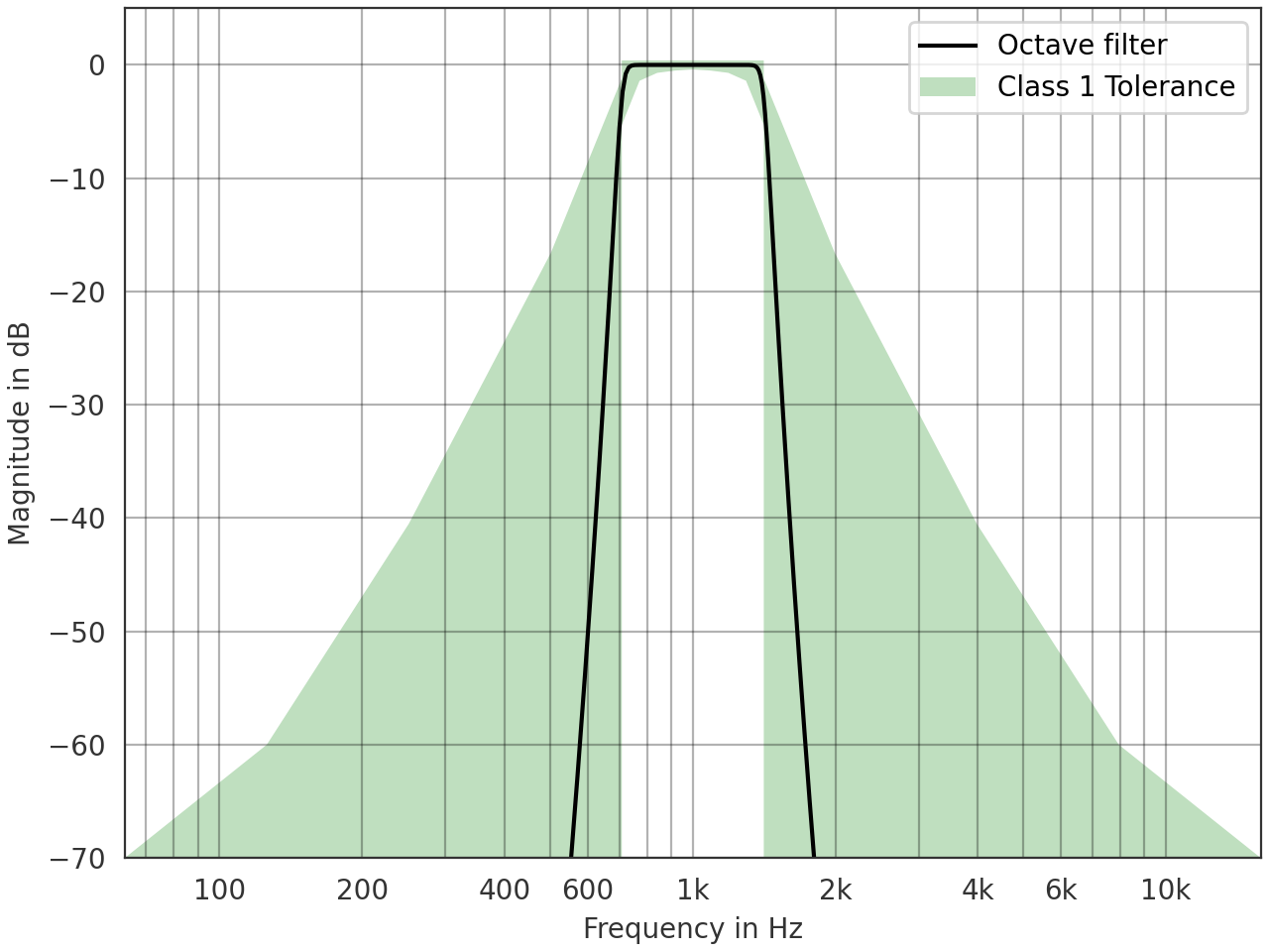
pyfar.constants.fractional_octave_filter_tolerance(exact_center_frequency: float, num_fractions: Literal[1, 3], tolerance_class: Literal[1, 2])

Calculate the tolerance limits for fractional octave band filters.

Calculation is in accordance with IEC 61260-1:2014 [10] (Section 5.10 and Table 1).

Note

The standard defines some lower tolerance limits as \(-\infty\), which is inconvenient for plotting. The returned tolerance is -60000 dB in these cases, which is below the smallest possible value of 20*np.log10(np.finfo(float).tiny \(\approx\)-6000 dB.

Parameters:

• exact_center_frequency (float) – The exact center frequency of the band filter in Hz (see fractional_octave_frequencies).

• num_fractions (Literal[1, 3]) – The number of bands an octave is divided into. 1 for octave bands and 3 for third octave bands.

• tolerance_class (Literal[1, 2]) – The tolerance class as defined in the standard. Must be 1 or 2.

Returns:

• lower_tolerance (numpy array) – Lower tolerance limits in dB of shape (19, ).

• upper_tolerance (numpy array) – Upper tolerance limits in dB of shape (19, ).

• frequencies (numpy array) – The frequencies in Hz at which the tolerance is given of shape (19, ).

References

[10]

IEC61260-1:2014 Octave-band and fractional-octave-band filters. Part 1: Specifications.

Examples

Class 1 tolerance region and filter for the 1000 Hz octave band.

>>> import pyfar as pf
>>> import matplotlib.pyplot as plt
>>>
>>> lower, upper, frequencies = \
...     pf.constants.fractional_octave_filter_tolerance(
...         exact_center_frequency=1000, num_fractions=1,
...         tolerance_class=1)
>>>
>>> octave_filter = pf.dsp.filter.fractional_octave_bands(
...     pf.signals.impulse(2**12), num_fractions=1,
...     frequency_range=(1000, 1000))
>>>
>>> ax = pf.plot.freq(octave_filter, color='k', label='Octave filter')
>>> plt.fill_between(
...     frequencies, lower, upper,
...     facecolor='g', alpha=.25, label='Class 1 Tolerance')
>>> ax.set_ylim(-70, 5)
>>> ax.set_xlim(63, 15_850)
>>> ax.legend()

(Source code, png, hires.png, pdf)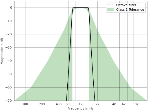

pyfar.constants.fractional_octave_frequencies_exact(num_fractions: int = 1, frequency_range: tuple[float, float] = (20, 20000.0))

Return the exact center and cutoff frequencies for fractional-octave-band filters.

The frequencies are calculated in accordance with the IEC 61260-1:2014 standard [11] (Sections 5.2, 5.3, 5.4 and 5.6).

The octave frequency ratio, \(G\), is given by the following expression.

\[G = 10^{\tfrac{3}{10}}\]

The center frequencies \(f_m\) are calculated using formula (1) for odd values of \(b\) and formula (2) for even values of \(b\).

(1)\[f_m = f_r \cdot G^{ \tfrac{x}{b}}\]

(2)\[f_m = f_r \cdot G^{ \tfrac{2x+1}{2b}}\]

where:

• \(b\) is the number of octave fractions.

• \(f_r\) is the reference frequency, set to 1000 Hz.

• \(x\) is the index of the frequency band.

Parameters:

• num_fractions (int, optional) – The number of bands an octave is divided into. E.g., 1 refers to octave bands and 3 to third octave bands. The default is 1. All positive integers are allowed.

• frequency_range (array, tuple) – The lower and upper frequency limits, the default is (20, 20e3).

Returns:

• center_frequencies (numpy.ndarray) – The exact center frequencies in Hz of the bandpass filters for each fractional octave band.

• lower_cutoff_frequencies (numpy.ndarray) – The lower cutoff frequencies in Hz of the bandpass filters for each fractional octave band.

• upper_cutoff_frequencies (numpy.ndarray) – The upper cutoff frequencies in Hz of the bandpass filters for each fractional octave band.

References

[11]

International Electrotechnical Commission, “IEC 61260-1:2014 - Electroacoustics - Octave-band and fractional-octave-band filters - Part 1: Specifications”, IEC, 2014.

Notes

The specified frequency_range is interpreted as frequencies lying within (fractional) octave bands defined by their cutoff frequencies (not their center frequencies). All bands that overlap with the specified frequency range are returned.

pyfar.constants.fractional_octave_frequencies_nominal(num_fractions: Literal[1, 3] = 1, frequency_range: tuple[float, float] = (20, 20000.0))

Return the nominal center frequencies for octave-band and one-third-octave-band filters.

Nominal center frequencies, as specified in the IEC 61260-1:2014 standard [12] (Section 5.5 and Annex E), are standardized values that approximate the exact center frequencies. They are defined from 10 Hz to 20 kHz.

Parameters:

• num_fractions ({1, 3}) – The number of octave fractions. 1 returns octave center frequencies, 3 returns third-octave center frequencies. The default is 1.

• frequency_range (array, tuple) – The lower and upper frequency limits, the default is (20, 20e3) following IEC 61260-1. E.g. (10, 20e3) would follow IEC 61672-1 [13].

Returns:

nominal – The nominal center frequencies.

Return type:

numpy.ndarray of float

Notes

The specified frequency_range is interpreted as frequencies lying within (fractional) octave bands defined by their cutoff frequencies (not their center frequencies). All bands that overlap with the specified frequency range are returned.

References

[12]

International Electrotechnical Commission, “IEC 61260-1:2014 - Electroacoustics - Octave-band and fractional-octave-band filters - Part 1: Specifications”, IEC, 2014.

[13]

International Electrotechnical Commission, “IEC 61672-1:2013 - Electroacoustics - Sound level meters - Part 1: Specifications”, IEC, 2013.

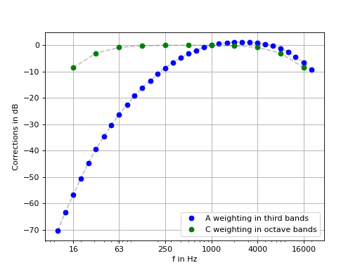
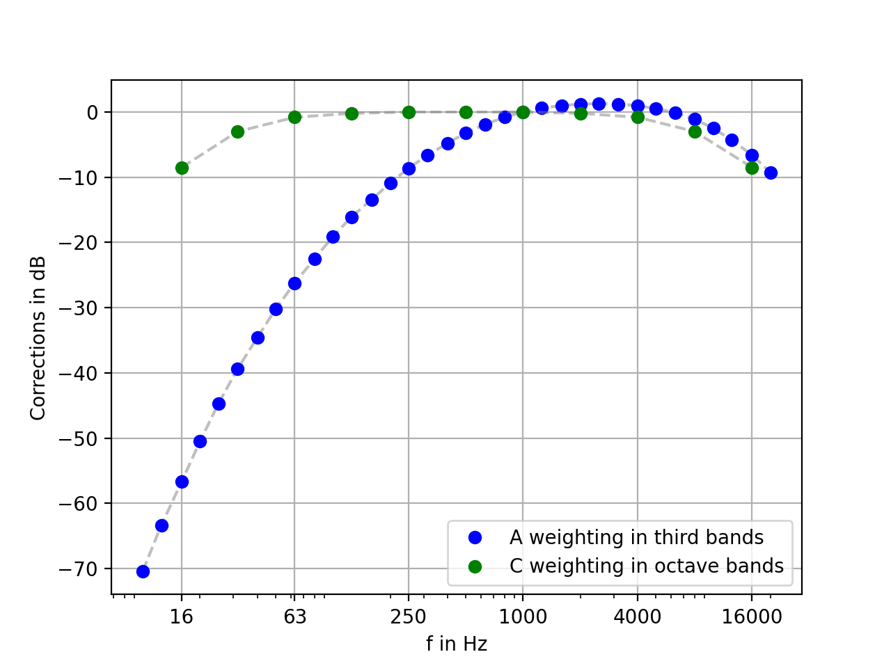
pyfar.constants.frequency_weighting_band_corrections(weighting: Literal['A', 'C'], num_fractions: Literal[1, 3], frequency_range: tuple[float, float])

Returns the A or C frequency weighting correction values for octave or third-octave bands in a given frequency range.

This function uses the nominal frequencies and their respective weights as given in the IEC 62672-1 standard [14].

Parameters:

• weighting (str ('A' or 'C')) – Which frequency weighting type to use.

• num_fractions ({1, 3}) – The number of octave fractions. 1 returns octave band corrections, 3 returns third-octave band corrections.

• frequency_range ((float, float)) – A range of what nominal center frequencies to include. The lowest defined center frequency is 10 Hz and the highest is 20 kHz.

Returns:

• nominal_frequencies (numpy.ndarray[float]) – The nominal center frequencies included in the given range.

• weights (numpy.ndarray[float]) – The correction values in dB for the specific frequency weighting.

References

[14]

International Electrotechnical Commission, “IEC 61672-1:2013 - Electroacoustics - Sound level meters - Part 1: Specifications”, IEC, 2013.

Examples

Plot the band correction levels.

>>> import pyfar as pf
>>> import matplotlib.pyplot as plt
>>> f_range = (10, 20000)
>>> nominals_third, weights_A = pf.constants.frequency_weighting_band_corrections(
...     "A", 3, f_range)
>>> nominals_octave, weights_C = pf.constants.frequency_weighting_band_corrections(
...     "C", 1, f_range)
>>> # plotting
>>> plt.plot(nominals_third, weights_A, "--", c=(0.5, 0.5, 0.5, 0.5))
>>> plt.plot(nominals_third, weights_A, "bo", label="A weighting in third bands")
>>> plt.plot(nominals_octave, weights_C, "--", c=(0.5, 0.5, 0.5, 0.5))
>>> plt.plot(nominals_octave, weights_C, "go", label="C weighting in octave bands")
>>> plt.legend()
>>> ticks = nominals_octave[::2].astype(int)
>>> plt.semilogx()
>>> plt.xticks(ticks, ticks)
>>> plt.xlabel("f in Hz")
>>> plt.ylabel("Corrections in dB")
>>> plt.grid()

(Source code, png, hires.png, pdf)

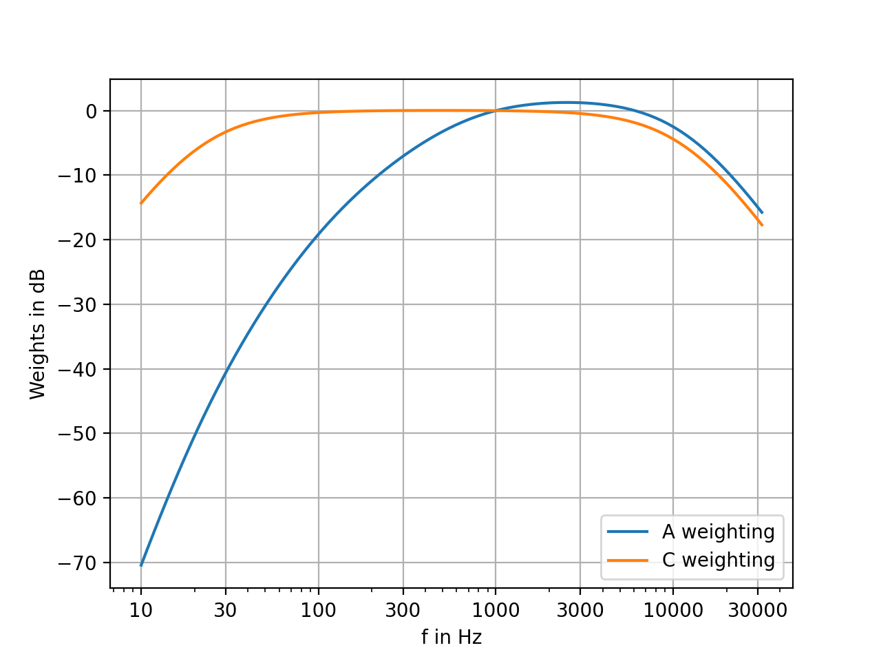
pyfar.constants.frequency_weighting_curve(weighting: Literal['A', 'C'], frequencies: list[float])

Calculates the level correction in dB of each frequency component when using the A or C frequency weighting.

Parameters:

• weighting (str ('A' or 'C')) – Which frequency weighting to use.

• frequencies (array-like) – The frequencies at which to evaluate the weighting curve.

Returns:

weights – The weights in dB in the same shape as frequencies. These weights are in accordance with IEC 61672-1 [15].

Return type:

numpy.ndarray[float]

References

[15]

International Electrotechnical Commission, “IEC 61672-1:2013 - Electroacoustics - Sound level meters - Part 1: Specifications”, IEC, 2013.

Examples

Plot the weighting curves.

>>> import pyfar as pf
>>> import matplotlib.pyplot as plt
>>> import numpy as np
>>> plot_frequencies = np.logspace(1, 4.5, 100, base=10)
>>> weights_A = pf.constants.frequency_weighting_curve(
...     "A", plot_frequencies)
>>> weights_C = pf.constants.frequency_weighting_curve(
...     "C", plot_frequencies)
>>> plt.plot(plot_frequencies, weights_A, label="A weighting")
>>> plt.plot(plot_frequencies, weights_C, label="C weighting")
>>> plt.semilogx()
>>> plt.xlabel("f in Hz")
>>> plt.ylabel("Weights in dB")
>>> ticks = [10, 30, 100, 300, 1000, 3000, 10000, 30000]
>>> plt.xticks(ticks, ticks)
>>> plt.grid()
>>> plt.legend()

(Source code, png, hires.png, pdf)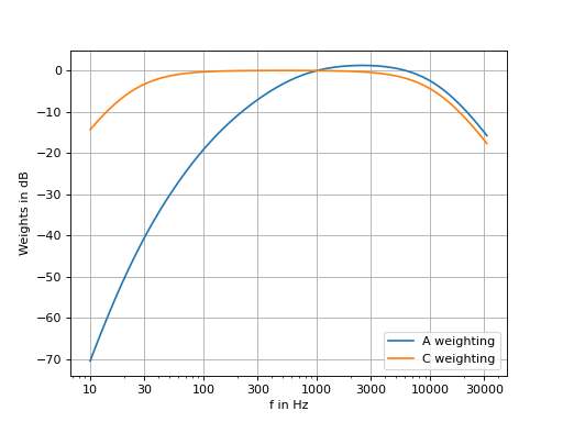

pyfar.constants.saturation_vapor_pressure_magnus(temperature)

Calculate the saturation vapor pressure of water in Pascal using the Magnus formula.

The Magnus formula is valid for temperatures between -45°C and 60°C [16].

\[e_s = 610.94 \cdot \exp\left(\frac{17.625 \cdot T}{T + 243.04}\right)\]

Parameters:

temperature (float, array_like) – Temperature in degrees Celsius (°C).

Returns:

p_sat – Saturation vapor pressure in Pa.

Return type:

float, array_like

References

[16]

O. A. Alduchov and R. E. Eskridge, “Improved Magnus Form Approximation of Saturation Vapor Pressure,” Journal of Applied Meteorology and Climatology, vol. 35, no. 4, pp. 60-609, Apr. 1996

pyfar.constants.speed_of_sound_cramer(temperature, relative_humidity, co2_ppm=425.19, atmospheric_pressure=None)

Calculate the speed of sound in air based on temperature, atmospheric pressure, humidity and CO₂ concentration.

This implements Cramers method described in [17].

Parameters:

• temperature (float, array_like) – Temperature in degree Celsius from 0°C to 30°C.

• relative_humidity (float, array_like) – Relative humidity in the range of 0 to 1.

• co2_ppm (float, array_like, optional) – CO₂ concentration in parts per million. The default is 425.19 ppm, based on [18]. Value must be below 10 000 ppm (1%).

• atmospheric_pressure (float, array_like, optional) – Atmospheric pressure in Pascal, by default reference_atmospheric_pressure. Value must be between 75 000 Pa to 102000 Pa.

Returns:

speed_of_sound – Speed of sound in air in m/s.

Return type:

float, array_like

References

[17]

O. Cramer, “The variation of the specific heat ratio and the speed of sound in air with temperature, pressure, humidity, and CO₂ concentration,” The Journal of the Acoustical Society of America, vol. 93, no. 5, pp. 2510-2516, May 1993, doi: 10.1121/1.405827.

[18]

Lan, X., Tans, P. and K.W. Thoning: Trends in globally-averaged CO2 determined from NOAA Global Monitoring Laboratory measurements. Version Friday, 14-Mar-2025 11:33:44 MDT https://doi.org/10.15138/9N0H-ZH07

pyfar.constants.speed_of_sound_ideal_gas(temperature, relative_humidity, atmospheric_pressure=None, saturation_vapor_pressure=None)

Calculate speed of sound in air using the ideal gas law.

The speed of sound in air can be calculated based on chapter 6.3 in [19]. All input parameters must be broadcastable to the same shape.

Parameters:

• temperature (float, array_like) – Temperature in degree Celsius.

• relative_humidity (float, array_like) – Relative humidity in the range of 0 to 1.

• atmospheric_pressure (float, array_like, optional) – Atmospheric pressure in Pascal, by default reference_atmospheric_pressure.

• saturation_vapor_pressure (float, array_like, optional) – Saturation vapor pressure in Pascal. If not given, the function saturation_vapor_pressure_magnus is used. Note that the valid temperature range therefore also depends on saturation_vapor_pressure_magnus.

Returns:

speed_of_sound – Speed of sound in air in m/s.

Return type:

float, array_like

References

[19]

V. E. Ostashev and D. K. Wilson, Acoustics in Moving Inhomogeneous Media, 2nd ed. London: CRC Press, 2015. doi: 10.1201/b18922.

pyfar.constants.speed_of_sound_simple(temperature)

Calculate the speed of sound in air using a simplified version of the ideal gas law based on the temperature.

The calculation follows ISO 9613-1 [20] (Formula A.5).

\[c(t) = c_\text{ref} \cdot \sqrt{\frac{t - t_0}{t_\text{ref} - t_0}}\]

where:

• \(t\) is the air temperature (°C)

• \(t_\text{ref}=20\mathrm{°C}\) is the reference air temperature (°C), see reference_air_temperature_celsius

• \(t_0=-273.15\) °C is the absolute zero temperature (°C), see absolute_zero_celsius

• \(c=343.2\) m/s is the speed of sound at the reference temperature, see reference_speed_of_sound

Parameters:

temperature (float, array_like) – Temperature in degree Celsius from -20°C to +50°C.

Returns:

speed_of_sound – Speed of sound in air in (m/s).

Return type:

float, array_like

References

[20]

ISO 9613-1:1993, Acoustics – Attenuation of sound during propagation outdoors – Part 1: Calculation of the absorption of sound by the atmosphere.